Page 55 - Finite Element Modeling and Simulations with ANSYS Workbench

40 Finite Element Modeling and Simulation with ANSYS Workbench

Substituting this into the second equation and rearranging, we have

 1 − 1u 2   
P
1260 × 10 5     =  
0 
 − 1 3  u 3    
Solving this, we obtain the displacements,
 u 2  1  3 P  .
0 01191 
  = 5   =   ()m
.

 u 3   2520 × 10  P   0 003968  
From the global FE equation, we can calculate the reaction forces,
 F X   0 − 0 5 . − 0 5 .   − 500
1
     
.
 F Y    0 − 0 5 . − 0.5 u 2     − −500  

1


5
 F Y  = 1260 × 10  0 0 0  u 3 =  00 .  (kN )

2
   − 1 . 1 5 . 0 5   v   −500 
3
 F X    3   
3 
 F Y    0 . 0 5 . 0 5    500  



Check the results!
A general MPC can be described as,
∑ Au j = 0
j
j
where A j ’s are constants and u j ’s are nodal displacement components. In FE software,
users only need to specify this relation to the software. The software will take care of
the solution process.
2.6 Case Study with ANSYS Workbench
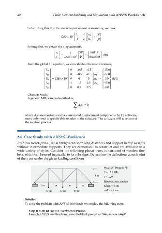
Problem Description: Truss bridges can span long distances and support heavy weights
without intermediate supports. They are economical to construct and are available in a
wide variety of styles. Consider the following planar truss, constructed of wooden tim-
bers, which can be used in parallel to form bridges. Determine the deflections at each joint
of the truss under the given loading conditions.

Solution
To solve the problem with ANSYS Workbench, we employ the following steps:

Step 1: Start an ANSYS Workbench Project
Launch ANSYS Workbench and save the blank project as ‘Woodtruss.wbpj’.