Page 54 - Finite Element Modeling and Simulations with ANSYS Workbench

Bars and Trusses 39

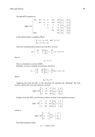
The global FE equation is,
 05 . 05 . 0 0 − 05 . − 05 . u 1   F 1X 
1
 − − −    
 15 . 0 1 05 . 05 .  1 v   F 1Y 
 1 0 − 1 0 u 2     F 
2X 

5
1260 × 10     =  
 1 0 0   2 v   F 2Y 
 15 05 u   F 

.
.
   3   3X 
5

  Sym. 0.5    v 3     F 3Y  
Load and boundary conditions (BCs):
u 1 = v 1 = v 2 = 0, and v 3 ′ = 0,
F X2 = , = 0.
P F x3 ′
From the transformation relation and the BCs, we have
 2 2  3 u  2
′ ν= −    = ( − 3 u + v ) = 0,
3
3
 2 2  3 v   2
that is,
u 3 − v 3 = 0
This is a multipoint constraint (MPC).
Similarly, we have a relation for the force at node 3,
 2 2  F X3  2
F x3 ′ =    = ( F X3 + F Y3 ) = 0,
 2 2  F Y3   2
that is,
F 3X + F 3Y = 0
Applying the load and BCs in the structure FE equation by “deleting” the first,
second, and fourth rows and columns, we have
 1 − 1 0 u 2   P 



5 
1260 × 10 − 1 1 5 . 0 5  u 3 = F  
.



3X

 0 0 5 . 0 5  v   F F Y3  
.
  3  
Further, from the MPC and the force relation at node 3, the equation becomes,
 1 − 1 0 u 2   P 

5 

1260 × 10 − 1 1 5 . 0 5  u 3 =   3 F X  
.



 0 0 5 . 0 5  u   
.
  3   − −F X3 
which is
 1 − 1  P 
 u

5 
1260 × 10 − 1 2  2   =  F X 
3 


 0 1   u 3    
3 
   −F X
The third equation yields,
F X3 =− 1260 × 10 5 u 3