Page 50 - Finite Element Modeling and Simulations with ANSYS Workbench

Bars and Trusses 35

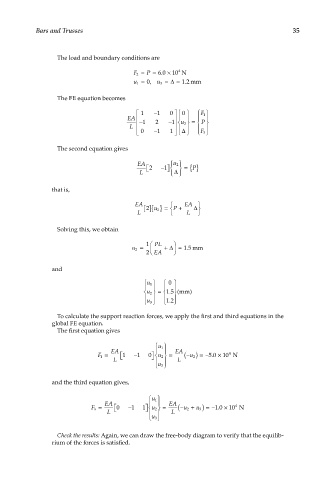
The load and boundary conditions are

4
F 2 = P = 60 × 10 N
.
u 1 = 0, u 3 = ∆ = 1 2 mm
.

The FE equation becomes
 1 − 1 0  0   F 1 

EA  − 1 2 − 1  u 2 =  
 

P

L   − 1  ∆   

 0 1    F 3 
The second equation gives
EA 2  − 1   u 2  P {}
 =
L    ∆  

that is,
EA 2 []{}  P + EA 
∆
u 2 = 

L  L 
Solving this, we obtain
1  PL 
u 2 =  + ∆  = 15 .mm
2  EA 

and
 u 1   0 
   
15  (mm
 u 2 =  . )
   12 . 
 u 3   
To calculate the support reaction forces, we apply the first and third equations in the
global FE equation.
The first equation gives

 u 1 

4
F 1 = EA  1  − 1 0   u 2 = EA − ( u 2) =− 5 0 × 10 N
.

L   L
 u 3 
and the third equation gives,
 u 1 
EA   EA
4
F 3 =  0  − 1 1  u 2 = − ( u 2 + ) =− 1 0 × 10 N
.

u 3
L   L
 u 3 
Check the results: Again, we can draw the free-body diagram to verify that the equilib-
rium of the forces is satisfied.