Page 105 - Fluid Power Engineering

Hydraulic Transmission Lines 79

Appendix 3B Modeling and Simulation of Hydraulic
Transmission Lines
This appendix deals with the development of lumped parameter
models and the simulation of a hydraulic transmission line. The model
takes into consideration the effects of the viscous friction, fluid inertia,
fluid compressibility, and elasticity of line material. The developed
models are one dimensional. The fluid speed and pressure are thought
of as averaged quantities over the cross section of the line. The sim-
plicity of the models results from the assumption of separate effects
of the previously mentioned parameters. The validity of the models
is evaluated by comparing the step response, calculated by the simu-
lation program, with experimental results.
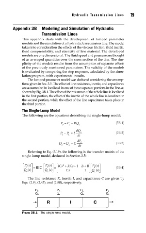
The lumped parameter model was deduced considering the assump-
tions given in Sec. 3.5. The effect of line resistance, inertia, and capacitance
are assumed to be localized in one of three separate portions in the line, as
shown by Fig. 3B.1. The effect of the resistance of the whole line is localized
in the first portion, the effect of the inertia of the whole line is localized in
the second portion, while the effect of the line capacitance takes place in
the third portion.

The Single-Lump Model
The following are the equations describing the single-lump model;

P − P = RQ (3B.1)
o 1 o
dQ
P − P = I o (3B.2)
1 L dt
dP
Q − Q = C L (3B.3)
o L dt
Referring to Eq. (3.19), the following is the transfer matrix of the
single-lump model, deduced in Section 3.5:

⎡ Ps ()⎤ ⎡ Ps ()⎤ ⎡ICs 2 + RCs 1 Is R ⎤
+
+ ⎤⎡Ps ()
⎢ o ⎥ = RIC ⎢ L ⎥ = ⎢ ⎥⎢ L ⎥ (3B.4)
⎣ Qs () ⎦ ⎣ Qs () ⎦ ⎣ Cs 1 ⎦⎣ Qs () ⎦
o
L
L
The line resistance R, inertia I, and capacitance C are given by
Eqs. (2.9), (2.47), and (2.80), respectively.

FIGURE 3B.1 The single-lump model.