Page 107 - Fluid Power Engineering

Hydraulic Transmission Lines 81

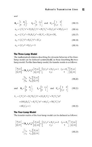
and

⎡ 1 R ⎤ ⎡ 1 Is⎤ ⎡ 1 0⎤
R = ⎢ 2 ⎥ , I = ⎢ 2 ⎥ and C = ⎢ ⎥ (3B.15)
2 2 2
⎣ 0 1 ⎦ ⎣ 0 1 ⎦ ⎣ Cs 1 ⎦
2
a = I Cs + 2 I R Cs + ( R C + 3 I C s +) 2 3 R Cs + 1 (3B.16)
2
2
24
23
2
11
2
2
2
2
2 2
2
2
2
2
2
2
a = I Cs + 3 I R Cs + ( R C + 2 I s 2+) R 2 (3B.17)
2
2
2
3
2
2
2
2
12
2
2
2
2
a = I C s + R C s + 2 C s (3B.18)
23
22
2
21
2
2
2
2
2
a 22 = I C s + R C s 1+ (3B.19)
2
2
2
2
The Three-Lump Model
The mathematical relations describing the dynamic behavior of the three-
lump model can be deduced systematically as those describing the two-
lump model. For the three-lump model, the transfer matrix is as follows:
3
⎡ Ps ()⎤ 3 Ps()⎡ ⎤ ⎡ ICs + R Cs + 1 I s R ⎤ ⎡Ps() ⎤
+
2
⎢ o ⎥ = [R I C ] L ⎥ = ⎢ ⎢ 3 3 3 3 3 3 ⎥ ⎢ L ⎥
3 ⎢
3 3
⎣ Qs () ⎦ ⎣ Qs() ⎦ ⎣ Cs 1 ⎦ ⎣ Qs() ⎦
o
3
L
L
⎡b b ⎤⎡Ps () ⎤
= ⎢ 11 12 ⎥⎢ L ⎥ (3B.20)
b
L
⎣ 21 b 22 ⎦⎣ Qs () ⎦
⎡ 1 R ⎤ ⎡ 1 Is⎤ ⎡ 1 0⎤
and R = 3 , I = 3 and C = (3B.21)
3 ⎢ ⎥ 3 ⎢ ⎥ 3 ⎢ ⎥
⎣ 0 1 ⎦ ⎣ 0 1 ⎦ ⎣ Cs 1 ⎦
3
b = I Cs + 3 I R Cs + ( 3 I R C + 5 I C ))s 4
2
3
2
2
2
36
35
3
11 3 3 3 3 3 3 3 3 3 3
2
3
+ (10IR C 2 + R C 3 )s 3 + (6I C + 5R C 2 )s 2
3 3 3 3 3 3 3 3 3
+ 6RCCs 1+ (3B.22)
3 3
The Four-Lump Model
The transfer matrix of the four-lump model can be deduced as follows:
⎡ Ps ()⎤ ⎡ Ps()⎤ ⎡ ICs + R Cs + 1 I s R ⎤ ⎡ Ps() ⎤
4
+
2
⎢ o ⎥ = [R I C ] 4 L ⎥ = ⎢ ⎢ 4 4 4 4 4 4 ⎥ ⎢ L ⎥
4 ⎢
⎣ Qs () ⎦ 4 4 ⎣ Qs() ⎦ ⎣ Cs 1 ⎦ ⎣ Qs() ⎦
o
L
L
4
= ⎡c 11 c 12 ⎤⎡Ps () ⎤ ⎥ (3B.23)
L
⎢
⎥⎢
c
L
⎣ 21 c 22 ⎦⎣ Qs () ⎦