Page 437 - Fluid-Structure Interactions Slender Structure and Axial Flow (Volume 1)

PIPES CONVEYING FLUID: NONLINEAR AND CHAOTIC DYNAMICS 409

10
0.0 0.1 0.2 0.3 0.4 0.5
/J

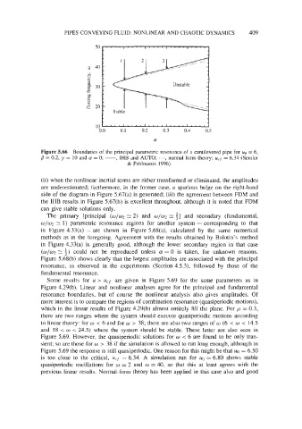
Figure 5.66 Boundaries of the principal parametric resonance of a cantilevered pipe for uo = 6,
= 0.2, y = 10 and a = 0; -, IHB and AUTO; . . ., normal form theory; ucf = 6.34 (Semler
& Paldoussis 1996).

(ii) when the nonlinear inertial terms are either transformed or eliminated, the amplitudes
are underestimated; furthermore, in the former case, a spurious bulge on the right-hand
side of the diagram in Figure 5.67(a) is generated; (iii) the agreement between FDM and
the IHB results in Figure 5.67(b) is excellent throughout, although it is noted that FDM
can give stable solutions only.
The primary [principal (w/% 21 2) and w/w2 2 t] and secondary (fundamental,
13/04 1) parametric resonance regions for another system - corresponding to that
2
in Figure 4.33(a) - are shown in Figure 5.68(a), calculated by the same numerical
methods as in the foregoing. Agreement with the results obtained by Bolotin's method
in Figure 4.33(a) is generally good, although the lower secondary region in that case
(w/w:! 2 i) could not be reproduced unless a = 0 is taken, for unknown reasons.
Figure 5.68(b) shows clearly that the largest amplitudes are associated with the principal
resonance, as observed in the experiments (Section 4.5.3), followed by those of the
fundamental resonance.
Some results for u > u,.. are given in Figure 5.69 for the same parameters as in
Figure 4.29(b). Linear and nonlinear analyses agree for the principal and fundamental
resonance boundaries, but of course the nonlinear analysis also gives amplitudes. Of
more interest is to compare the regions of combination resonance (quasiperiodic motions),
which in the linear results of Figure 4.29(b) almost entirely fill the plane. For = 0.3,
there are two ranges where the system should execute quasiperiodic motions according
to linear theory: for w < 6 and for w > 38; there are also two ranges of w (6 < w < 14.5
and 18 -= w -= 24.5) where the system should be stable. These latter are also seen in
Figure 5.69. However, the quasiperiodic solutions for w < 6 are found to be only tran-
sient; so are those for w > 38 if the simulation is allowed to run !ong enough, although in
Figure 5.69 the response is still quasiperiodic. One reason for this might be that ug = 6.50
is too close to the critical, ucf = 6.34. A simulation run for uo = 6.80 shows stable
quasiperiodic oscillations for w = 2 and w = 40, so that this at least agrees with the
previous linear results. Normal-form theory has been applied in this case also and good