Page 39 - T. Anderson-Fracture Mechanics - Fundamentals and Applns.-CRC (2005)

1656_C01.fm Page 19 Tuesday, April 12, 2005 5:55 PM

History and Overview 19

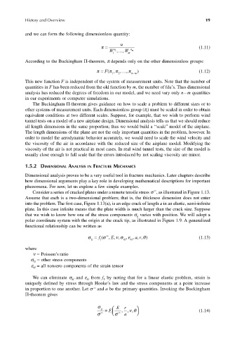
and we can form the following dimensionless quantity:
u
π = (1.11)
W a 1 , W , a m
1 m
According to the Buckingham Π-theorem, π depends only on the other dimensionless groups:

π π = F(, π , π , ) (1.12)
−
1 2 nm
This new function F is independent of the system of measurement units. Note that the number of
quantities in F has been reduced from the old function by m, the number of fdu’s. Thus dimensional
analysis has reduced the degrees of freedom in our model, and we need vary only n – m quantities
in our experiments or computer simulations.
The Buckingham Π-theorem gives guidance on how to scale a problem to different sizes or to
other systems of measurement units. Each dimensionless group (π ) must be scaled in order to obtain
i
equivalent conditions at two different scales. Suppose, for example, that we wish to perform wind
tunnel tests on a model of a new airplane design. Dimensional analysis tells us that we should reduce
all length dimensions in the same proportion; thus we would build a ‘‘scale” model of the airplane.
The length dimensions of the plane are not the only important quantities in the problem, however. In
order to model the aerodynamic behavior accurately, we would need to scale the wind velocity and
the viscosity of the air in accordance with the reduced size of the airplane model. Modifying the
viscosity of the air is not practical in most cases. In real wind tunnel tests, the size of the model is
usually close enough to full scale that the errors introduced by not scaling viscosity are minor.

1.5.2 DIMENSIONAL ANALYSIS IN FRACTURE MECHANICS

Dimensional analysis proves to be a very useful tool in fracture mechanics. Later chapters describe
how dimensional arguments play a key role in developing mathematical descriptions for important
phenomena. For now, let us explore a few simple examples.
Consider a series of cracked plates under a remote tensile stress σ ∞ , as illustrated in Figure 1.13.
Assume that each is a two-dimensional problem; that is, the thickness dimension does not enter
into the problem. The first case, Figure 1.13(a), is an edge crack of length a in an elastic, semi-infinite
plate. In this case infinite means that the plate width is much larger than the crack size. Suppose
that we wish to know how one of the stress components σ varies with position. We will adopt a
ij
polar coordinate system with the origin at the crack tip, as illustrated in Figure 1.9. A generalized
functional relationship can be written as

σ ij f 1 σ = ( ∞ , ν σ E kl ε , , kl r , , , ) (1.13)
θ a ,
where
ν = Poisson’s ratio
σ = other stress components
kl
ε = all nonzero components of the strain tensor
kl
We can eliminate σ and ε from f by noting that for a linear elastic problem, strain is
kl
kl
1
uniquely defined by stress through Hooke’s law and the stress components at a point increase
∞
in proportion to one another. Let σ and a be the primary quantities. Invoking the Buckingham
Π-theorem gives
σ ij E  r 
a
σ ∞ = F 1  σ ∞ ,, νθ ,  (1.14)