Page 38 - T. Anderson-Fracture Mechanics - Fundamentals and Applns.-CRC (2005)

1656_C01.fm Page 18 Tuesday, April 12, 2005 5:55 PM

18 Fracture Mechanics: Fundamentals and Applications

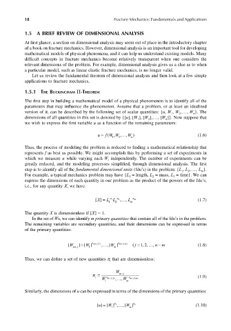
1.5 A BRIEF REVIEW OF DIMENSIONAL ANALYSIS

At first glance, a section on dimensional analysis may seem out of place in the introductory chapter
of a book on fracture mechanics. However, dimensional analysis is an important tool for developing
mathematical models of physical phenomena, and it can help us understand existing models. Many
difficult concepts in fracture mechanics become relatively transparent when one considers the
relevant dimensions of the problem. For example, dimensional analysis gives us a clue as to when
a particular model, such as linear elastic fracture mechanics, is no longer valid.
Let us review the fundamental theorem of dimensional analysis and then look at a few simple
applications to fracture mechanics.

1.5.1 THE BUCKINGHAM Π-THEOREM

The first step in building a mathematical model of a physical phenomenon is to identify all of the
parameters that may influence the phenomenon. Assume that a problem, or at least an idealized
version of it, can be described by the following set of scalar quantities: {u, W , W ,…, W }. The
n
2
1
dimensions of all quantities in this set is denoted by {[u], [W ], [W ],…, [W ]}. Now suppose that
n
2
1
we wish to express the first variable u as a function of the remaining parameters:
u f = ( W W , , W , ) (1.6)
1 2 n
Thus, the process of modeling the problem is reduced to finding a mathematical relationship that
represents f as best as possible. We might accomplish this by performing a set of experiments in
which we measure u while varying each W independently. The number of experiments can be
i
greatly reduced, and the modeling processes simplified, through dimensional analysis. The first
step is to identify all of the fundamental dimensional units (fdu’s) in the problem: {L , L ,…, L }.
m
1
2
For example, a typical mechanics problem may have {L = length, L = mass, L = time}. We can
3
1
2
express the dimensions of each quantity in our problem as the product of the powers of the fdu’s;
i.e., for any quantity X, we have
X
[] = L a L a 1 2 , , L a m (1.7)
1 2 m
The quantity X is dimensionless if [X] = 1.
In the set of Ws, we can identify m primary quantities that contain all of the fdu’s in the problem.
The remaining variables are secondary quantities, and their dimensions can be expressed in terms
of the primary quantities:

=
m
1
[ W mj ] [ W 1 ] a mj+ () ,  ,[ W m ] a mj+ ( ) ( j = , , , n 12 − m (1.8)
+
Thus, we can define a set of new quantities π that are dimensionless:
i
W
+
π = mj (1.9)
i
W
1 a mj+ , , W m a mj m+ 1 () ( )
Similarly, the dimensions of u can be expressed in terms of the dimensions of the primary quantities:

u
=
[] [ W ] , ,[ W ] a m (1.10)
a 1
1 m