Page 130 - Fundamentals of Communications Systems

4.6 Chapter Four

Complex Baseband to Bandpass to Complex
Bandpass Conversion Baseband Conversion
x (t)
1
x (t) LPF x (t)
I
I
+
2 cos( 2πft) Σ x (t) 2 cos( 2πft)
c
c
c
−
π 2 π 2
x (t)
2
x (t) −x (t)
Q LPF Q
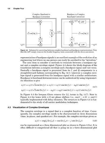
Figure 4.4 Schemes for converting between complex baseband and bandpass representations. Note
that the LPF simply removes the double frequency term associated with the down conversion.

representation of bandpass signals is an excellent example of the evolution of an
engineering tool where no one person can really be ascribed to the “invention.”
The next item to consider is methods to translate between a bandpass sig-
nal and a complex envelope signal. Figure 4.4 shows the block diagram of the
translation between a complex envelope and a bandpass signal and vice versa.
Basically a bandpass signal is generated from its I and Q components in a
straightforward fashion corresponding to Eq. (4.1). Likewise a complex enve-
lope signal is generated from the bandpass signal with a similar architecture.
Bandpass to baseband downconversion can be understood by using trigonomet-
ric identities to give
√
x 1 (t) = x c (t) 2 cos(2π f c t) = x I (t) + x I (t) cos(4π f c t) − x Q (t) sin(4π f c t)
(4.7)
√
x 2 (t) = x c (t) 2 sin(2π f c t) =−x Q (t) + x Q (t) cos(4π f c t) + x I (t) sin(4π f c t)

In Figure 4.4 the lowpass filters remove the 2 f c terms in Eq. (4.7). Note in
Figure 4.4 the boxes with π/2 are phase shifters (i.e., cos(θ − π/2) = sin(θ))
typically implemented with delay elements. The structure in Figure 4.4 is fun-
damental to the study of all carrier modulation techniques.

4.3 Visualization of Complex Envelopes
The complex envelope is a signal that is a complex function of time. Conse-
quently, the complex envelope needs to be characterized in three dimensions
(time, in-phase, and quadrature). For example, the complex envelope given as
x z (t) = exp[ j 2π f m t] = cos(2π f m t) + j sin(2π f m t) (4.8)
can be represented as a three dimensional plot as shown in Figure 4.5(a). It is
often difficult to comprehend all that is going on in a three-dimensional plot