Page 132 - Fundamentals of Communications Systems

4.8 Chapter Four

and it will be used often in future sections of this text. The vector diagram first
gained utility in the days when the standard tool for examining the time domain
characteristics of a communication signal was the dual channel analog oscillo-
scope. To produce a vector diagram with a dual channel oscilloscope, x I (t) is put
into one channel and x Q (t) is put into the second channel and the scope is con-
figured to plot channel 1 versus channel 2. Since early test instruments could
simply generate this visualization, the vector diagram has traditionally found
utility in engineering practice. In fact, modern communication test equipment
like the Agilent 89600 vector signal analyzer are based around the characteri-
zation of the complex envelope and have the ability to measure vector diagrams
of bandpass signals.

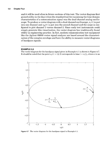
EXAMPLE 4.2
The vector diagram for the bandpass signal given in Example 4.1 is shown in Figure 4.7.
It should be noted that the point x z (t) = (2, 0) corresponds to time t = n/f m where nis an

2

1.5

1

0.5
t = n
f m
x Q (t) 0

t = n + 3
−0.5
f f 4
m m
−1

−1.5

−1
−2 −1.5 −1 −0.5 0 0.5 1 1.5 2
x (t)
I
Figure 4.7 The vector diagram for the bandpass signal in Example 4.1.