Page 136 - Fundamentals of Communications Systems

4.12 Chapter Four

EXAMPLE 4.4
(Example 4.1 cont.)
x I (t) = 2 cos(2π f m t) x Q (t) = sin(2π f m t)
1 1
X I (f ) = δ(f − f m ) + δ(f + f m ) X Q (f ) = δ(f − f m ) − δ(f + f m )
2 j 2 j
X z (f ) = X I (f ) + jX Q (f ) = 1.5δ(f − f m ) + 0.5δ(f + f m )
and using Eq. (4.14) gives the bandpass signal spectrum as

1.5 1 1.5 1
X c (f ) = √ δ(f − f c − f m ) + √ δ(f − f c + f m ) + √ δ(f + f c + f m ) + √ δ(f + f c − f m )
2 2 2 2 2 2
Note in this example B T = 2 f m

EXAMPLE 4.5
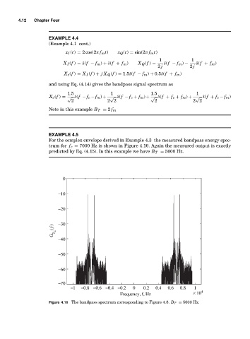
For the complex envelope derived in Example 4.3 the measured bandpass energy spec-
trum for f c = 7000 Hz is shown in Figure 4.10. Again the measured output is exactly
predicted by Eq. (4.15). In this example we have B T = 5000 Hz.

0

−10

−20

G y C ( f ) −30

−40

−50

−60

−70
−1 −0.8 −0.6 −0.4 −0.2 0 0.2 0.4 0.6 0.8 1
Frequency, f, Hz × 10 4
Figure 4.10 The bandpass spectrum corresponding to Figure 4.8. B T = 5000 Hz.