Page 141 - Fundamentals of Communications Systems

Complex Baseband Representation of Bandpass Signals 4.17

This produces
f
⎧
⎪ 2 − −f m ≤ f ≤ f m
f m
⎪
⎪
1 f m ≤ f ≤ 2 f m
⎨
H z (f ) = (4.37)
⎪ 3 −2 f m ≤ f ≤−f m
⎪
⎪
0 elsewhere
⎩
and now the Fourier transform of the complex envelope of the filter output is
Y z (f ) = H z (f )X z (f ) = 1.5δ(f − f m ) + 1.5δ(f + f m ) (4.38)
The complex envelope and bandpass signal are given as
√
y z (t) = 3 cos(2π f m t) y c (t) = 3 cos(2π f m t) 2 cos(2π f c t) (4.39)

In other words, convolving the complex envelope of the input signal with the
complex envelope of the filter response produces the complex envelope of the
output signal. The different scale factor was introduced in Eq. (4.26) so that
Eq. (4.35) would have a familiar form. This result is significant since y c (t) can
be derived by computing a convolution of baseband (complex) signals, which is
generally much simpler than computing the bandpass convolution. Since x z (t)
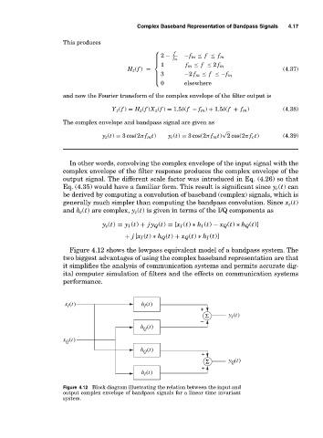
and h z (t) are complex, y z (t) is given in terms of the I/Q components as
y z (t) = y I (t) + jy Q (t) = [x I (t) ∗ h I (t) − x Q (t) ∗ h Q (t)]

+ j [x I (t) ∗ h Q (t) + x Q (t) ∗ h I (t)]
Figure 4.12 shows the lowpass equivalent model of a bandpass system. The
two biggest advantages of using the complex baseband representation are that
it simplifies the analysis of communication systems and permits accurate dig-
ital computer simulation of filters and the effects on communication systems
performance.

x (t) h (t)
I
I
+
Σ y (t)
I
−
h (t)
Q
x (t)
Q
h (t)
Q
+
Σ y (t)
Q
+
h (t)
I
Figure 4.12 Block diagram illustrating the relation between the input and
output complex envelope of bandpass signals for a linear time invariant
system.