Page 193 - Fundamentals of Communications Systems

Amplitude Modulation 6.15

the transmitted signal phase is always zero. The received signal has the form
y z (t) = A c (1 + aβ sin(2π f m (t − τ p ))) exp[ j φ p ] (6.16)

The vector diagram for the noiseless received signal, y z (t), is plotted in Figure 6.17(a).
By examining this figure it is clear that the phase shift has rotated the complex en-
velope but not changed the amplitude of the signal. This is evident in the plots of the
transmitted and received amplitude and phase (measured in radians) signals shown in
Figure 6.17(b). The received amplitude signal and the transmitted amplitude signal are
different only by a time delay, τ p . The received phase is exactly φ p .

EXAMPLE 6.7
Consider the LC-AM computer-generated voice signal given in Example 6.6 with a
carrier frequency of 7 kHz and a propagation delay in the channel of 45.6 µs.
◦
This results in a φ p =−114 (see Example 6.4.) The plot of the envelope of the re-
ceived signal,

2
2
y A (t) = y (t) + y (t)
I Q
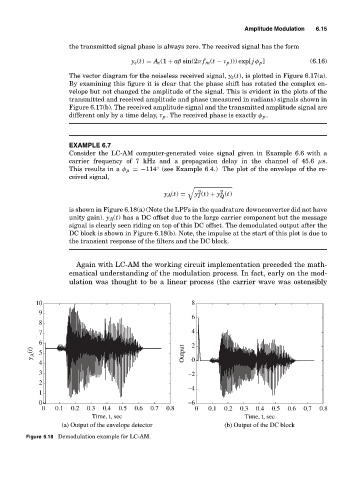
is shown in Figure 6.18(a) (Note the LPFs in the quadrature downconverter did not have
unity gain). y A (t) has a DC offset due to the large carrier component but the message
signal is clearly seen riding on top of this DC offset. The demodulated output after the
DC block is shown in Figure 6.18(b). Note, the impulse at the start of this plot is due to
the transient response of the filters and the DC block.

Again with LC-AM the working circuit implementation preceded the math-
ematical understanding of the modulation process. In fact, early on the mod-
ulation was thought to be a linear process (the carrier wave was ostensibly

10 8
9
6
8
7 4
6 2
y A (t) 5 Output

4 0
3 −2
2
−4
1
0 −6
0 0.1 0.2 0.3 0.4 0.5 0.6 0.7 0.8 0 0.1 0.2 0.3 0.4 0.5 0.6 0.7 0.8
Time, t, sec Time, t, sec
(a) Output of the envelope detector (b) Output of the DC block
Figure 6.18 Demodulation example for LC-AM.