Page 146 - Fundamentals of Probability and Statistics for Engineers

Functions of Random Variables 129

y

y
2 y =g(x)
y
y
1
x
x = g (y) x = g (y) x = g (y)
–1
–1
–1
1 1 2 2 3 3

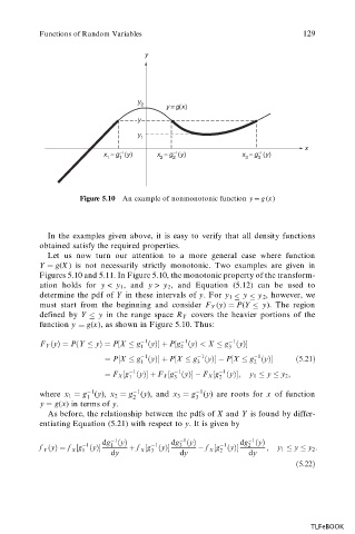
Figure 5.10 An example of nonmonotonic function y g (x)

ˆ
In the examples given above, it is easy to verify that all density functions
obtained satisfy the required properties.
Let us now turn our attention to a more general case where function
Y ˆ g(X ) is not necessarily strictly monotonic. Two examples are given in
Figures 5.10 and 5.11. In Figure 5.10, the monotonic property of the transform-
ation holds for y < y 1 , and y > y 2 , and Equation (5.12) can be used to
determine the pdf of Y in these intervals of y. For y 1 y 2 y , however, we
must start from the beginning and consider F Y (y) ˆ P(Y y). The region
defined by Y y in the range space R Y covers the heavier portions of the
function y ˆ g(x), as shown in Figure 5.10. Thus:

1

1

1
F Y y†ˆ P Y y†ˆ P‰X g y†Š ‡ P‰g y† < X g y†Š
1 2 3

1

1

1
ˆ P‰X g y†Š ‡ P‰X g y†Š
P‰X g y†Š 5:21†
3
2
1

1

1

1
ˆ F X ‰g y†Š ‡ F X ‰g y†Š
F X ‰g y†Š; y 1 y y 2 ;
1 3 2

1

1

1
where x 1 ˆ g y), x 2 ˆ g y),and x 3 ˆ g y) are roots for x of function
1 2 3
( ) in terms of . y
y ˆ g x
As before, the relationship between the pdfs of X and Y is found by differ-
entiating Equation (5.21) with respect to y. It is given by

1

1

1
dg y† dg y† dg y†

1

1

1
f y†ˆ f ‰g y†Š 1 dy ‡ f ‰g y†Š 3 dy
f ‰g y†Š 2 dy ; y 1 y y 2 :
3
X
Y
X
X
1
2
5:22†
TLFeBOOK