Page 147 - Fundamentals of Probability and Statistics for Engineers

130 Fundamentals of Probability and Statistics for Engineers

y

1

y

x

–1

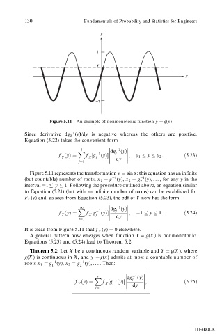
Figure 5.11 An example of nonmonotonic function y ˆ g(x)

1
)/
Since derivative dg (y) dy is negative whereas the others are positive,
2
Equation (5.22) takes the convenient form

3
1
j
X
1 dg y†
f y†ˆ f ‰g y†Š ; y 1 y y 2 : 5:23†

Y
j
X
jˆ1 dy
Figure 5.11 represents the transformation y ˆ sin x; this equation has an infinite

1
1
(but countable) number of roots, x 1 ˆ g (y), x 2 ˆ g (y), . . . , for any y in the
1
2

interval 1 y 1. Following the procedure outlined above, an equation similar
to Equation (5.21) (but with an infinite number of terms) can be established for
F Y (y) and, as seen from Equation (5.23), the pdf of Y now has the form
1
1
j
X
1 dg y†
f y†ˆ f ‰g y†Š ;
1 y 1: 5:24†

j
X
Y
jˆ1 dy
It is clear from Figure 5.11 that f (y) ˆ 0 elsewhere.
Y
A general pattern now emerges when function Y ˆ g(X ) is nonmonotonic.
Equations (5.23) and (5.24) lead to Theorem 5.2.

Theorem 5.2: Let X be a continuous random variable and Y ˆ g(X ), where

g(X ) is continuous in X, and y ˆ g(x) admits at most a countable number of

1
roots x 1 ˆ
1 ˆ g (y), ... . Then:
g (y), x 2
1 2

r
1
j
X
1 dg y†
f y†ˆ ; 5:25†

j
Y f ‰g y†Š dy
X
jˆ1
TLFeBOOK