Page 167 - Fundamentals of Probability and Statistics for Engineers

150 Fundamentals of Probability and Statistics for Engineers

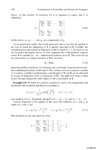
where r is the number of solutions for x of equation y ˆ g( x), and J j is
defined by
qg qg qg

1
1
1
j1 j1

j1

qy 1 qy 2
qy n
. .
. . 5:69†

. .
J j ˆ

1
1
qg qg qg
1
jn jn

jn

qy 1 qy 2 qy n
In the above, g j1 , g j2 ,... , and g jn are components of g .
j
As we mentioned earlier, the results presented above can also be applied to
the case in which the dimension of Y is smaller than that of X. Consider the
transformation represented in Equation (5.60) in which m < n. In order to use
the formulae developed above, we first augment the m-dimensional random
vector Y by another (n
m) – dimensional random vector Z. The vector Z can

be constructed as a simple function of X in the form
Z ˆ h X†; 5:70†
where h satisfies conditions of continuity and continuity in partial derivatives.
On combining Equations (5.60) and (5.70), we have now an n-random-variable
to n-random-variable transformation, and the jpdf of Y and Z can be obtained

by means of Equation (5.67) or Equation (5.68). The jpdf of Y alone is then
found through integration with respect to the components of Z.
Example 5.18. Problem: let random variables X 1 and X 2 be independent and

identically and normally distributed according to
1
x 2 1
f x 1 †ˆ exp ;
1 < x 1 < 1;
X 1 1=2
2 † 2
and similarly for X 2 . Determine the jpdf of Y 1 ˆ X 1 ‡ X 2 , and Y 2 ˆ X 1
X 2 .
Answer: Equation (5.67) applies in this case. The solutions of x 1 and x 2 in
terms of y 1 and y 2 are

1

1
x 1 ˆ g y†ˆ y 1 ‡ y 2 ; x 2 ˆ g y†ˆ y 1
y 2 : 5:71†
1 2 2 2
The Jacobian in this case takes the form

1
qg 1 qg
1 1
1 1

1
qy 1 2 2
qy 2 ˆ ˆ
:
J ˆ
1
qg qg
1 1 1 2
2
2
2 2

qy 1 qy 2

TLFeBOOK