Page 267 - Fundamentals of Probability and Statistics for Engineers

250 Fundamentals of Probability and Statistics for Engineers

Returning now to the chemical yield example, the frequency diagram as
shown in Figure 8.1 has the familiar properties of a probability density function
(pdf). Hence, probabilities associated with various events can be estimated. For
example, the probability of a batch having less than 68% yield can be read off
from the frequency diagram by summing over the areas to the left of 68%,
0 01 ‡ :
:
giving 0.13 (0 02 ‡ : 0 025 ‡ :
0 075). Similarly, the probability of a batch
0 035 ‡ :
0 01). Let
having yields greater than 72% is 0.18 (0 105 ‡ : 0 03 ‡ : us
:
remember, however, these are probabilities calculated based on the observed
data. A different set of data obtained from the same chemical process would
in general lead to a different frequency diagram and hence different values for
these probabilities. Consequently, they are, at best, estimates of probabilities
P(X < 68) and P(X > 72) associated with the underlying random variable X.
A remark on the choice of the number of intervals for plotting the histograms
and frequency diagrams is in order. For this example, the choice of 12 intervals is
convenient on account of the range of values spanned by the observations and of
the fact that the resulting resolution is adequate for calculations of probabilities
carried out earlier. In Figure 8.3, a histogram is constructed using 4 intervals
instead of 12 for the same example. It is easy to see that it projects quite a different,
and less accurate, visual impression of data behavior. It is thus important to
choose the number of intervals consistent with the information one wishes to
extract from the mathematical model. As a practical guide, Sturges (1926) suggests
that an approximate value for the number of intervals, k, be determined from

k ˆ 1 ‡ 3:3 log n; 8:1†
10
where n is the sample size.
From the modeling point of view, it is reasonable to select a normal distribution
as the probabilistic model for percentage yield X by observing that its random vari-
ations are the resultant of numerous independent random sources in the chem-
ical manufacturing process. Whether or not this is a reasonable selection can be

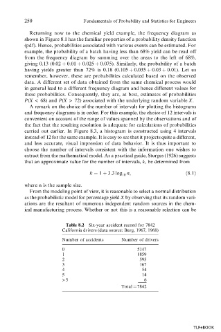
Table 8.2 Six-year accident record for 7842
California drivers (data source: Burg, 1967, 1968)
Number of accidents Number of drivers
0 5147
1 1859
2 595
3 167
4 54
5 14
>5 6
Total ˆ 7842

TLFeBOOK