Page 271 - Fundamentals of Probability and Statistics for Engineers

254 Fundamentals of Probability and Statistics for Engineers

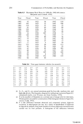
Table 8.3 Maximum flood flows (in 1000 cfs), 1902–60 (source:
Benjamin and Cornell, 1970).
Year Flood Year Flood Year Flood

1902 42 1922 36 1942 110
1903 102 1923 22 1943 108
1904 118 1924 42 1944 25
1905 81 1925 64 1945 60
1906 128 1926 56 1946 54
1907 230 1927 94 1947 46
1908 16 1928 185 1948 37
1909 140 1929 14 1949 17
1910 31 1930 80 1950 46
1911 75 1931 12 1951 92
1912 16 1932 23 1952 13
1913 17 1933 9 1953 59
1914 122 1934 20 1954 113
1915 81 1935 59 1955 55
1916 42 1936 85 1956 203
1917 80 1937 19 1957 83
1918 28 1938 185 1958 102
1919 66 1939 8 1959 35
1920 23 1940 152 1960 135
1921 62 1941 84

Table 8.4 Time gaps between vehicles (in seconds)
4.1 3.5 2.2 2.7 2.7 4.1 3.4 1.8 3.1 2.1
2.1 1.7 2.3 3.0 4.1 3.2 2.2 2.3 1.5 1.1
2.5 4.7 1.8 4.8 1.8 4.0 4.9 3.1 5.7 5.7
3.1 2.0 2.9 5.9 2.1 3.0 4.4 2.1 2.6 2.7
3.2 2.5 1.7 2.0 2.7 1.2 9.0 1.8 2.1 5.4
2.1 3.8 4.5 3.3 2.1 2.1 7.1 4.7 3.1 1.7
2.2 3.1 1.7 3.1 2.3 8.1 5.7 2.2 4.0 2.7
1.5 1.7 4.0 6.4 1.5 2.2 1.2 5.1 2.7 2.4
1.7 1.2 2.7 7.0 3.9 5.2 2.7 3.5 2.9 1.2
1.5 2.7 2.9 4.1 3.1 1.9 4.8 4.0 3.0 2.7

(i) X 1 , X 2 , and X 3 are annual premiums paid by low-risk, medium-risk, and
high-risk drivers. The frequency diagram for each group is given in Figure 8.5.
(simulated results, over 50 years, are from Ferreira, 1974).
(j) X is the number of blemishes in a certain type of image tube for television,
58 data points are used for construction of the histogram shown in Figure 8.6.
(source: Link, 1972).
(k) X is the difference between observed and computed urinary digitoxin
excretion, in micrograms per day. In a study of metabolism of digitoxin
to digoxin in patients, long-term studies of urinary digitoxin excretion were
carried out on four patients. A histogram of the difference between

TLFeBOOK