Page 197 - Fundamentals of Radar Signal Processing

obtained by an inverse DFT of those frequency samples is the original slow-

time signal replicated at intervals of K samples. Recall that y [m] is confined to
s
the interval [0, M – 1]. If K ≥ M, y [m – qK] = 0 in the interval of interest [0, K–
s
1] for all q ≠ 0, so that ŷ [m] = y [m]. This is the usual case where the DFT size
s
s
is at least as long as the data sequence size.
The Nyquist rate for sampling in the frequency dimension is now apparent.
If K ≥ M the original slow-time signal y [m] is not aliased by the frequency
s
domain sampling operation. Consequently, it can be recovered from the
replicated signal ŷ [m] implied by the sampled spectrum by simply excising the
s
principal period m ∈ [0, K – 1]. This is the equivalent of the lowpass filter
required to reconstruct a sampled time-domain signal; the time and frequency
domains have simply been reversed in this discussion of sampling in the
frequency domain.
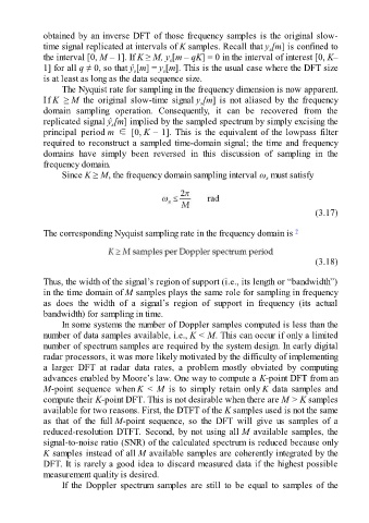
Since K ≥ M, the frequency domain sampling interval ω must satisfy
s

(3.17)

The corresponding Nyquist sampling rate in the frequency domain is 7

(3.18)

Thus, the width of the signal’s region of support (i.e., its length or “bandwidth”)
in the time domain of M samples plays the same role for sampling in frequency
as does the width of a signal’s region of support in frequency (its actual
bandwidth) for sampling in time.

In some systems the number of Doppler samples computed is less than the
number of data samples available, i.e., K < M. This can occur if only a limited
number of spectrum samples are required by the system design. In early digital
radar processors, it was more likely motivated by the difficulty of implementing
a larger DFT at radar data rates, a problem mostly obviated by computing
advances enabled by Moore’s law. One way to compute a K-point DFT from an

M-point sequence when K < M is to simply retain only K data samples and
compute their K-point DFT. This is not desirable when there are M > K samples
available for two reasons. First, the DTFT of the K samples used is not the same
as that of the full M-point sequence, so the DFT will give us samples of a
reduced-resolution DTFT. Second, by not using all M available samples, the
signal-to-noise ratio (SNR) of the calculated spectrum is reduced because only
K samples instead of all M available samples are coherently integrated by the

DFT. It is rarely a good idea to discard measured data if the highest possible
measurement quality is desired.
If the Doppler spectrum samples are still to be equal to samples of the