Page 201 - Fundamentals of Radar Signal Processing

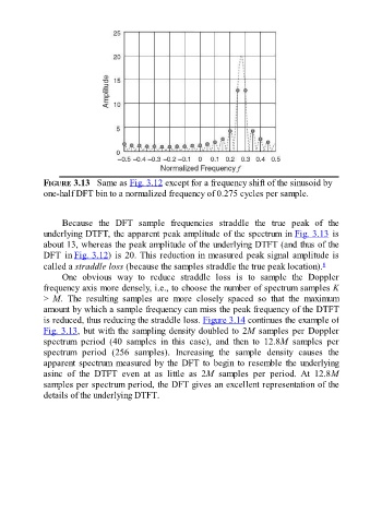
FIGURE 3.13 Same as Fig. 3.12 except for a frequency shift of the sinusoid by
one-half DFT bin to a normalized frequency of 0.275 cycles per sample.

Because the DFT sample frequencies straddle the true peak of the
underlying DTFT, the apparent peak amplitude of the spectrum in Fig. 3.13 is
about 13, whereas the peak amplitude of the underlying DTFT (and thus of the
DFT in Fig. 3.12) is 20. This reduction in measured peak signal amplitude is

called a straddle loss (because the samples straddle the true peak location). 8
One obvious way to reduce straddle loss is to sample the Doppler
frequency axis more densely, i.e., to choose the number of spectrum samples K
> M. The resulting samples are more closely spaced so that the maximum
amount by which a sample frequency can miss the peak frequency of the DTFT

is reduced, thus reducing the straddle loss. Figure 3.14 continues the example of
Fig. 3.13, but with the sampling density doubled to 2M samples per Doppler
spectrum period (40 samples in this case), and then to 12.8M samples per
spectrum period (256 samples). Increasing the sample density causes the
apparent spectrum measured by the DFT to begin to resemble the underlying
asinc of the DTFT even at as little as 2M samples per period. At 12.8M
samples per spectrum period, the DFT gives an excellent representation of the

details of the underlying DTFT.