Page 198 - Fundamentals of Radar Signal Processing

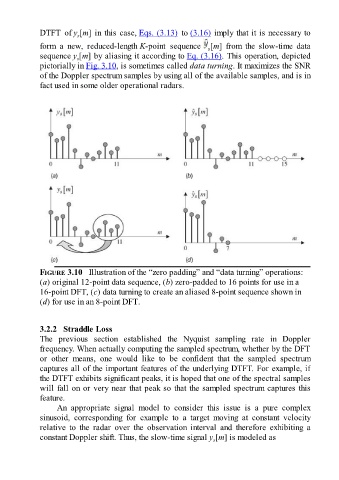
DTFT of y [m] in this case, Eqs. (3.13) to (3.16) imply that it is necessary to
s
form a new, reduced-length K-point sequence [m] from the slow-time data
s
sequence y [m] by aliasing it according to Eq. (3.16). This operation, depicted
s
pictorially in Fig. 3.10, is sometimes called data turning. It maximizes the SNR
of the Doppler spectrum samples by using all of the available samples, and is in
fact used in some older operational radars.

FIGURE 3.10 Illustration of the “zero padding” and “data turning” operations:
(a) original 12-point data sequence, (b) zero-padded to 16 points for use in a
16-point DFT, (c) data turning to create an aliased 8-point sequence shown in
(d) for use in an 8-point DFT.

3.2.2 Straddle Loss
The previous section established the Nyquist sampling rate in Doppler
frequency. When actually computing the sampled spectrum, whether by the DFT
or other means, one would like to be confident that the sampled spectrum
captures all of the important features of the underlying DTFT. For example, if
the DTFT exhibits significant peaks, it is hoped that one of the spectral samples
will fall on or very near that peak so that the sampled spectrum captures this
feature.

An appropriate signal model to consider this issue is a pure complex
sinusoid, corresponding for example to a target moving at constant velocity
relative to the radar over the observation interval and therefore exhibiting a
constant Doppler shift. Thus, the slow-time signal y [m] is modeled as
s