Page 202 - Fundamentals of Radar Signal Processing

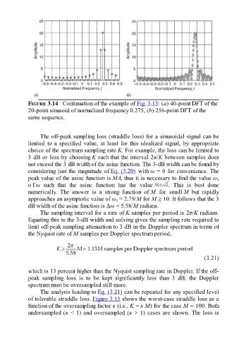
FIGURE 3.14 Continuation of the example of Fig. 3.13: (a) 40-point DFT of the

20-point sinusoid of normalized frequency 0.275, (b) 256-point DFT of the
same sequence.

The off-peak sampling loss (straddle loss) for a sinusoidal signal can be
limited to a specified value, at least for this idealized signal, by appropriate
choice of the spectrum sampling rate K. For example, the loss can be limited to
3 dB or less by choosing K such that the interval 2π/Κ between samples does
not exceed the 3 dB width of the asinc function. The 3-dB width can be found by
considering just the magnitude of Eq. (3.20) with ω = 0 for convenience. The
peak value of the asinc function is MA, thus it is necessary to find the value ω 3

o f ω such that the asinc function has the value . This is best done
numerically. The answer is a strong function of M for small M but rapidly
approaches an asymptotic value of ω = 2.79/M for M ≥ 10. It follows that the 3
3
dB width of the asinc function is Δω = 5.58/M radians.
The sampling interval for a rate of K samples per period is 2π/Κ radians.

Equating this to the 3-dB width and solving gives the sampling rate required to
limit off-peak sampling attenuation to 3 dB in the Doppler spectrum in terms of
the Nyquist rate of M samples per Doppler spectrum period,

(3.21)

which is 13 percent higher than the Nyquist sampling rate in Doppler. If the off-

peak sampling loss is to be kept significantly less than 3 dB, the Doppler
spectrum must be oversampled still more.
The analysis leading to Eq. (3.21) can be repeated for any specified level
of tolerable straddle loss. Figure 3.15 shows the worst-case straddle loss as a
function of the oversampling factor κ (i.e., K = κ M) for the case M = 100. Both
undersampled (κ < 1) and oversampled (κ > 1) cases are shown. The loss is