Page 257 - Fundamentals of Radar Signal Processing

in this case the expected slow-time signal is simply a constant. A matched filter

for a Doppler-shifted pulse burst can be implemented by continuing to use the
single-pulse matched filter in fast time and constructing the appropriate slow-
time matched filter for the signal expected for a given Doppler shift.
Suppose the normalized Doppler shift of interest is ω radians per sample.
D
The expected slow-time signal is then of the form Aexp(jω m). After
D
conjugation and time-reversal the slow-time matched filter coefficients will be

h[m] = exp(+jω m). Consider the response of this filter when the actual
D
Doppler shift of the signal is ω. The matched filter peak output occurs when the
impulse response and data sequence are fully overlapped, giving

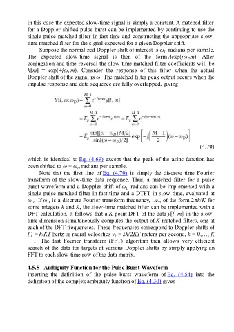
(4.70)

which is identical to Eq. (4.69) except that the peak of the asinc function has
been shifted to ω = ω radians per sample.
D
Note that the first line of Eq. (4.70) is simply the discrete time Fourier
transform of the slow-time data sequence. Thus, a matched filter for a pulse
burst waveform and a Doppler shift of ω radians can be implemented with a
D
single-pulse matched filter in fast time and a DTFT in slow time, evaluated at

ω . If ω is a discrete Fourier transform frequency, i.e., of the form 2πk/K for
D
D
some integers k and K, the slow-time matched filter can be implemented with a
DFT calculation. It follows that a K-point DFT of the data y[l, m] in the slow-
time dimension simultaneously computes the output of K-matched filters, one at
each of the DFT frequencies. These frequencies correspond to Doppler shifts of

F = k/KT hertz or radial velocities v = λk/2KT meters per second, k = 0,…, K
k
k
– 1. The fast Fourier transform (FFT) algorithm then allows very efficient
search of the data for targets at various Doppler shifts by simply applying an
FFT to each slow-time row of the data matrix.

4.5.5 Ambiguity Function for the Pulse Burst Waveform
Inserting the definition of the pulse burst waveform of Eq. (4.54) into the
definition of the complex ambiguity function of Eq. (4.30) gives