Page 46 - Fundamentals of Radar Signal Processing

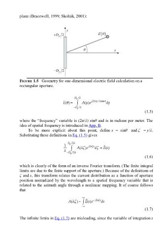
plane (Bracewell, 1999; Skolnik, 2001):

FIGURE 1.5 Geometry for one-dimensional electric field calculation on a

rectangular aperture.

(1.5)

where the “frequency” variable is (2π/λ) sinθ and is in radians per meter. The
idea of spatial frequency is introduced in App. B.
To be more explicit about this point, define s = sinθ and ζ = y/λ.

Substituting these definitions in Eq. (1.5) gives

(1.6)

which is clearly of the form of an inverse Fourier transform. (The finite integral
limits are due to the finite support of the aperture.) Because of the definitions of

ζ and s, this transform relates the current distribution as a function of aperture
position normalized by the wavelength to a spatial frequency variable that is
related to the azimuth angle through a nonlinear mapping. It of course follows
that

(1.7)

The infinite limits in Eq. (1.7) are misleading, since the variable of integration s