Page 136 - Fundamentals of The Finite Element Method for Heat and Fluid Flow

STEADY STATE HEAT CONDUCTION IN MULTI-DIMENSIONS
128
Γ q k Γ h Insulated Insulated
i j

Insulated
Γ T
Exposed to boundary
conditions
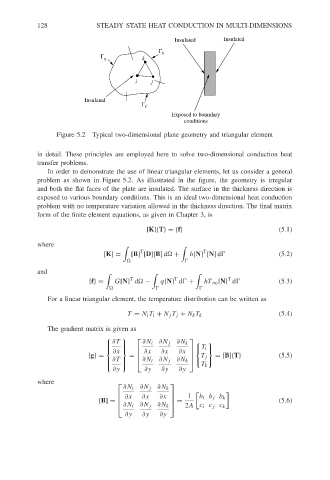
Figure 5.2 Typical two-dimensional plane geometry and triangular element

in detail. These principles are employed here to solve two-dimensional conduction heat
transfer problems.
In order to demonstrate the use of linear triangular elements, let us consider a general
problem as shown in Figure 5.2. As illustrated in the figure, the geometry is irregular
and both the flat faces of the plate are insulated. The surface in the thickness direction is
exposed to various boundary conditions. This is an ideal two-dimensional heat conduction
problem with no temperature variation allowed in the thickness direction. The final matrix
form of the finite element equations, as given in Chapter 3, is

[K]{T}={f} (5.1)
where
T T
[K] = [B] [D][B]d
+ h[N] [N]d (5.2)

and
T T T
{f}= G[N] d
− q[N] d + hT ∞ [N] d (5.3)

For a linear triangular element, the temperature distribution can be written as

T = N i T i + N j T j + N k T k (5.4)

The gradient matrix is given as
∂T ∂N i ∂N j ∂N k
   
   
 
∂x  ∂x ∂x ∂x 
  T i 
{g}= =   T j = [B]{T} (5.5)
 ∂N i ∂N j ∂N k 
 ∂T   
  T k
∂y ∂y ∂y ∂y
 
where
 
∂N i ∂N j ∂N k
∂x ∂x ∂x 1
  b i b j b k
[B] =   = (5.6)
 ∂N i ∂N j ∂N k
2A c i c j c k

∂y ∂y ∂y