Page 138 - Fundamentals of The Finite Element Method for Heat and Fluid Flow

STEADY STATE HEAT CONDUCTION IN MULTI-DIMENSIONS
130
where x o and y o are the coordinates of the point source. In the above equations, all the
∗
shape function values must be evaluated at (x o ,y o ) (note that although G is a point source,
in two dimensions, it is a line source in the thickness direction and expressed in units of
W/m). The contribution from the point source is then appropriately distributed to the three
nodes of the element that contains the point source.
In order to demonstrate the characteristics of two-dimensional steady state heat transfer,
the temperature distribution in a flat plate having constant temperature boundary conditions
is considered in the following example.
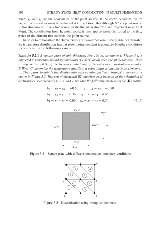
Example 5.2.1 A square plate of unit thickness, size 100 cm, as shown in Figure 5.4, is
subjected to isothermal boundary conditions of 100 C on all sides except the top side, which
◦
◦
is subjected to 500 C. If the thermal conductivity of the material is constant and equal to
10 W/m C, determine the temperature distribution using linear triangular finite elements.
◦
The square domain is first divided into eight equal-sized linear triangular elements, as
shown in Figure 5.5. Two sets of elemental [K] matrices exist because of the orientation of
the triangles. For elements 1, 3, 5, and 7, we have the following elements of the [K] matrix:
b 1 = y 2 − y 4 =−0.50; c 1 = x 4 − x 2 =−0.50
b 2 = y 4 − y 1 = 0.50; c 2 = x 1 − x 4 = 0.00

b 4 = y 1 − y 2 = 0.00; c 4 = x 2 − x 1 = 0.50 (5.11)

500°C

100°C 1 m
100°C

100°C
1 m
Figure 5.4 Square plate with different temperature boundary conditions

7 8 9

6 8
5 7
4 5 6
2 4
1
3
1 2 3
Figure 5.5 Discretization using triangular elements