Page 137 - Fundamentals of The Finite Element Method for Heat and Fluid Flow

STEADY STATE HEAT CONDUCTION IN MULTI-DIMENSIONS
Note that G in Equation 5.3 is a uniform heat source. Assuming an anisotropic material,
we have

k x 0 129
[D] = (5.7)
0 k y
Note that the off-diagonal terms are neglected from the above equation for the sake of
simplicity. Substituting [D] and [B] into Equation 5.2, we get, for a boundary element as
shown in Figure 5.3
  2   2   
b b i b j b i b k c 00 0
t  i 2 i c i c j c i c k  htl jk
2
[K] e = k x  b i b j b j b j b k  + k y  c i c j c j c j c k  +  02 1  (5.8)
4A  2 2  6
b i b k b j b k b c i c k c j c k c 01 2
k k
The subscript e in the above equation denotes a single element. It should be noted that
in the above equation, d
is equal to tdA and d is equal to tdl,where t is the thickness
of the plate and l is the length of an element side on the domain boundary. In a similar
fashion, the forcing vector can be written as
     
GAt 1 qtl ij 1 hT a tl jk 0
{f} e = 1 − 1 + 1 (5.9)
2
1 0 1
3   2    
The integration formulae used for the above equations are simple, as indicated in
Chapter 3. For convenience, we have listed the integration formulae in Appendix B.
As seen in the previous equations, the effect of uniform heat generation contributes to
all three nodes of an element, irrespective of its position. However, the convection and flux
boundary conditions are applicable only on the boundaries of the domain.
∗
If we need to have a ‘point source’ G instead of a ‘uniform source’ G,the first term
in Equation 5.9 is replaced with
 
N i 
{f}= G t N j (5.10)
∗
 
N k
(x o ,y o )
k
h, T a

G

j
i
q

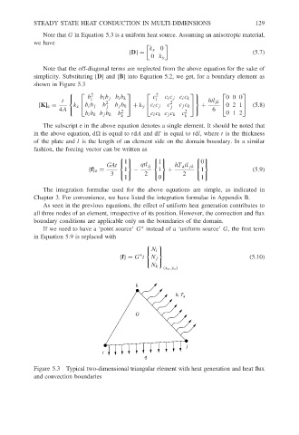
Figure 5.3 Typical two-dimensional triangular element with heat generation and heat flux
and convection boundaries