Page 140 - Fundamentals of The Finite Element Method for Heat and Fluid Flow

STEADY STATE HEAT CONDUCTION IN MULTI-DIMENSIONS
132
where w is the width, H is the height of the plate, T top is the temperature at the top side
and T side is the temperature at the other sides of the plate. Therefore,
◦
T(0.5, 0.5) = 200.11 C (5.19)
As seen, the finite element solution is in close agreement with the analytical solution. It
is interesting to note that the finite difference solution is given by
T 2 + T 4 + T 6 + T 8
◦
T 5 = = 200 C (5.20)
4
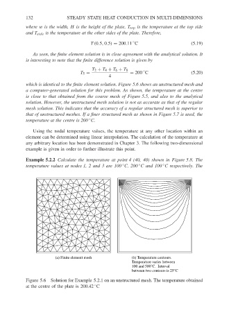
which is identical to the finite element solution. Figure 5.6 shows an unstructured mesh and
a computer-generated solution for this problem. As shown, the temperature at the centre
is close to that obtained from the coarse mesh of Figure 5.5, and also to the analytical
solution. However, the unstructured mesh solution is not as accurate as that of the regular
mesh solution. This indicates that the accuracy of a regular structured mesh is superior to
that of unstructured meshes. If a finer structured mesh as shown in Figure 5.7 is used, the
temperature at the centre is 200 C.
◦
Using the nodal temperature values, the temperature at any other location within an
element can be determined using linear interpolation. The calculation of the temperature at
any arbitrary location has been demonstrated in Chapter 3. The following two-dimensional
example is given in order to further illustrate this point.

Example 5.2.2 Calculate the temperature at point 4 (40, 40) shown in Figure 5.8. The
◦
◦
temperature values at nodes 1, 2 and 3 are 100 C, 200 C and 100 C respectively. The
◦

(a) Finite element mesh (b) Temperature contours.
Temperature varies between
100 and 500°C. Interval
between two contours is 25°C
Figure 5.6 Solution for Example 5.2.1 on an unstructured mesh. The temperature obtained
at the centre of the plate is 200.42 C
◦