Page 144 - Fundamentals of The Finite Element Method for Heat and Fluid Flow

STEADY STATE HEAT CONDUCTION IN MULTI-DIMENSIONS
136
and


 5.0
{f} 2 = 95.0 (5.30)
95.0
 
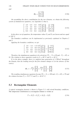
On assembling the above contributions for the two elements, we obtain the following
system of simultaneous equations, (see Appendix C) that is,
2.0 −1.0 −1.0
     
0.0 T 1
−2.0
   
T 2
 −1.0 2.0 0.0 −1.0     6.0 
  = (5.31)
−1.0 0.0 4.0

 0.0 T 3 91.0
   

 
0.0 −1.0 0.0 4.0 T 4 95.0

In the above set of equations, the temperature values T 2 and T 4 are known and are equal
to 100 C.
◦
The boundary conditions can be implemented as previously explained in Chapters 2
and 3.
Applying the boundary conditions, we get
     
 −2.0 
2.0 −1.0 −1.00.0 T 1
   
0.0 1.0 0.00.0    100.0 
  T 2
  = (5.32)
−1.0 0.0
 
4.00.0 T 3
 91.0
   
0.0 0.0 0.01.0    100.0 
T 4
Therefore, the simultaneous equations to be solved are 2T 1 − T 3 = 98 and −T 1 + 4T 3 =
◦
91. The solution to these equations results in T 1 = 69 C and T 3 = 40 C.
◦
3
If, in the above example, there is a uniform heat generation of 1.2 W/cm throughout
the domain, then the loading term for the first element changes to (in the absence of line
source)
     
ql 31 1 GAt 1 0
{f} 1 =− 0 + 1 = 5 (5.33)
1 1 0
2   3    
The resulting simultaneous equations become 2T 1 − T 3 = 100 and −T 1 + 4T 3 = 95 and
◦
the solution becomes T 1 = 70.71 C and T 3 = 40.42 C.
◦
5.3 Rectangular Elements
A typical rectangular element is shown in Figure 5.11 with mixed boundary conditions.
The temperature distribution in a rectangular element is written as
T = N i T i + N j T j + N k T k + N l T l (5.34)