Page 148 - Fundamentals of The Finite Element Method for Heat and Fluid Flow

STEADY STATE HEAT CONDUCTION IN MULTI-DIMENSIONS
140
q
j j t h, T a
t
k t i
i
k
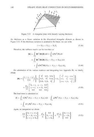
Figure 5.13 A triangular plate with linearly varying thickness

the thickness as a linear variation in the discretized triangular element as shown in
Figure 5.13. If the thickness variation is assumed to be linear, we can write
t = N i t i + N j t j + N k T k (5.48)

Therefore, the stiffness matrix can be rewritten as

T T
[K] = [B] [D][B]d
+ h[N] [N]dS

S

T
= [B] [D][B](N i t i + N j t j + N k t k ) dA
A

T
+ h[N] [N](N i t i + N j t j + N k t k ) dl ik (5.49)
l
On substitution of the various matrices and integrating (see Appendix B), we finally
obtain
b c
  2   2 
i b i b j b i b k i c i c j c i c k 
t i + t j + t k  2 2
[K] = k x  b i b j b j b j b k  + k y  c i c j c j c j c k 
12A  2 2 
b i b k b j b k b c i c k c j c k c
k k
3t i + t j t i + t j 0.0
 
hl ij
+  t i + t j t i + 3t j 0.0  (5.50)
12
0.0 0.0 0.0
The load term is calculated as

T T
{f}= G[N] (N i t i + N j t j + N k t k ) dA − q[N] (N i t i + N j t j + N k t k ) dl jk
A l jk

T
+ hT a [N] (N i t i + N j t j + N k t k ) dl ij (5.51)
l ij
Again, on integration we obtain
     
GA 2t i + t j + t k ql jk  0.0  hT a l ij 2t i + t j
t i + 2t j + t k − 2t j + t k + t i + 2t j (5.52)
6
12   6    
t i + t j + 2t k t j + 2t k 0.0