Page 149 - Fundamentals of The Finite Element Method for Heat and Fluid Flow

STEADY STATE HEAT CONDUCTION IN MULTI-DIMENSIONS
If the thickness is constant, the above relations reduce to the same set of equations as
in Section 5.2.
5.5 Three-dimensional Problems 141

The formulation of a three-dimensional problem follows a similar approach as explained
previously for two-dimensional plane geometries but with an additional third dimension.
The finite element equation is the same as in Equation 5.1, that is,

[K]{T}={f} (5.53)

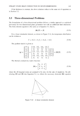
For a linear tetrahedral element, as shown in Figure 5.14, the temperature distribution
can be written as

T = N i T i + N j T j + N k T k + N l T l (5.54)

The gradient matrix is given as
∂T ∂N i ∂N j ∂N k ∂N l
   
 
   
∂x ∂x ∂x ∂x
 
   
 ∂x  T i 
     
∂T  ∂N i ∂N j ∂N k ∂N l  T j
   
{g}= =   = [B]{T} (5.55)
 ∂y ∂y ∂y  T

 ∂y  ∂y   k 
  
   
∂N i ∂N j ∂N k ∂N l T l
   
∂T 
 
 
∂z ∂z ∂z ∂z ∂z
The thermal conductivity matrix becomes
 
k x 00
[D] =  0 k y 0  (5.56)
00 k z
where the off-diagonal terms are assumed to be zero, for the sake of simplicity. On sub-
stituting [D] and [B] into Equation 5.2, we obtain the necessary elemental [K] equation
l

k
i
j

Figure 5.14 A linear tetrahedral element