Page 154 - Fundamentals of The Finite Element Method for Heat and Fluid Flow

STEADY STATE HEAT CONDUCTION IN MULTI-DIMENSIONS
146
It is possible to approximately recover the two-dimensional plane problem by substi-
tuting a very large value for the radius r. In order to clarify the axisymmetric formulation,
an example problem is solved as follows.
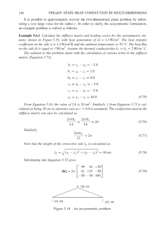
Example 5.6.1 Calculate the stiffness matrix and loading vector for the axisymmetric ele-
3
ment, shown in Figure 5.18, with heat generation of G = 1.2 W/cm . The heat transfer
2
coefficient on the side ij is 1.2 W/cm K and the ambient temperature is 30 C. The heat flux
◦
2
on the side jk is equal to 1 W/cm . Assume the thermal conductivities k r = k z = 2 W/cm C.
◦
The solution to this problem starts with the calculation of various terms in the stiffness
matrix (Equation 5.72).
b i = z j − z k =−2.0
b j = z k − z i = 2.0
b k = z i − z j = 0.0
c i = x k − x j =−5.0

c j = x i − x k =−5.0
c k = x j − x i = 10.0 (5.75)
2
From Equation 5.63, the value of 2A is 20 cm . Similarly, r from Equation 5.73 is cal-
culated as being 20 cm (a reference axis at r = 0.0 is assumed). The coefficients used in the
stiffness matrix can also be calculated as
2πrk r 2πrk z
= = 2π (5.76)
4A 4A
Similarly,
2πhl ij
= 2π (5.77)
12
Note that the length of the convective side l ij is calculated as

2
2
l ij = (x i − x j ) + (y i − y j ) = 10 cm (5.78)
Substituting into Equation 5.72 gives
99 61 −50
 
[K] = 2π  61 119 −50  (5.79)
−50 −50 100

k (20, 12)

i (15, 10) j (25, 10)

Figure 5.18 An axisymmetric problem