Page 150 - Fundamentals of The Finite Element Method for Heat and Fluid Flow

STEADY STATE HEAT CONDUCTION IN MULTI-DIMENSIONS
142
500 °C (top)
100 °C (side)
1 m Insulated

x 2
1 m 1 m
100 °C (side) x 3
x 1

100 °C (bottom)
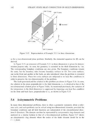
Figure 5.15 Representation of Example 5.2.1 in three dimensions

as for a two-dimensional plane problem. Similarly, the elemental equation for {f} can be
derived.
In Figure 5.15, an extension of Example 5.2.1 to three dimensions is given for demon-
stration purpose only. As seen, the geometry is extended in the third dimension by 1 m.
The corresponding boundary conditions are also given. The boundary conditions remain
the same, but the boundary sides become boundary surfaces in 3D. Two extra surfaces,
one in the front and another at the back, are also introduced when the problem is extended
to three dimensions. These two extra surfaces are subjected to no heat flux conditions in
order to preserve the two-dimensionality of the problem.
The mesh generated and the solution to this problem are shown in Figure 5.16. As seen,
the solution in the plane perpendicular to the third dimension, x 3 , is identical to that of the
two-dimensional solution given in Figure 5.6(b). As mentioned previously, the variation of
the temperature in the third dimension is suppressed by imposing a no heat flux condition
on the front and back faces, perpendicular to x 3 , as shown in Figure 5.15.

5.6 Axisymmetric Problems

In many three-dimensional problems, there is often a geometric symmetry about a refer-
ence axis, and such problems can be solved using two-dimensional elements, provided the
boundary conditions and all field functions are independent of the circumferential direc-
tion (θ direction). The domain can then be represented by axisymmetric ring elements and
analysed in a similar fashion to that of a two-dimensional problem. Figure 5.17 shows
an axisymmetric ring element where the nodes of the finite element model lie in the
r − z plane.