Page 146 - Fundamentals of The Finite Element Method for Heat and Fluid Flow

STEADY STATE HEAT CONDUCTION IN MULTI-DIMENSIONS
138
After integration, the matrix [K] becomes

2.0 −2.0 −1.0 1.0   2.0 −2.0 −1.0 1.0 
−2.0 2.0 1.0 −1.0 −2.0 2.0 1.0 −1.0
k x a   k y b  
[K] =   +  
6b  −1.0 1.0 2.0 −2.0  6a  −1.0 1.0 2.0 −2.0 
1.0 −1.0 −2.0 2.0 1.0 −1.0 −2.0 2.0
0.00.00.00.0
 
0.00.00.00.0 
hl 
+   (5.40)
12  0.00.04.02.0 
0.00.02.04.0
The loading vector can be written as
   
N i  1
2b 2a    

 

T N j GAt 1
{f}= G[N] dA = G dx dy = (5.41)
0 0 N k  4 1
 


   
N l 1
The heat flux and convective heat transfer boundary integrals are evaluated as for
triangular elements. In order to demonstrate the application of such elements, Example
5.2.3 will now be reconsidered using a rectangular element.
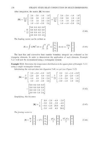
Example 5.3.1 Determine the temperature distribution in the square plate of Example 5.2.3,
using a single rectangular element.
Substituting the relevant data into Equation 5.40, we get (see Figure 5.12)
   
2.0 −2.0 −1.0 1.0 2.0 1.0 −1.0 −2.0
−2.0 2.0 1.0 −1.0 1.0 2.0 −2.0 −1.0
5   5  
[K] =   +  
15  −1.0 1.0 2.0 −2.0  15  −1.0 −2.0 2.0 1.0 
1.0 −1.0 −2.0 2.0 −2.0 −1.0 1.0 2.0
0.00.00.00.0
 
0.00.00.00.0
 
+   (5.42)
0.00.02.01.0
 
0.00.01.02.0
Simplifying, this becomes
8.0 −2.0 −4.0 −2.0
 
−2.0 8.0 −2.0 −4.0
1  
[K] =   (5.43)
6  −4.0 −2.0 20.0 4.0 
−2.0 −4.0 4.0 20.0
The forcing vector is
       
1 N 1 1 0
 
6t    N 2  qtl 14   hT a tl 31  
 
 


0
1
0
∗
{f}= + G t − + (5.44)
2 2
4 1 N 3 0 1
       
1 N 4 1 1
       