Page 29 - Fundamentals of The Finite Element Method for Heat and Fluid Flow

SOME BASIC DISCRETE SYSTEMS
where h is the heat transfer coefficient and T a is the ambient temperature. We can rearrange
the previous three equations as follows:
k 1 A k 1 A 21
T 1 − T 2 = qA
L 1 L 1
k 1 A k 1 A k 2 A k 2 A
− T 1 + + T 2 − T 3 = 0
L 1 L 1 L 2 L 2
k 2 A k 2 A
− T 2 + + hA T 3 = hAT a (2.11)
L 2 L 2
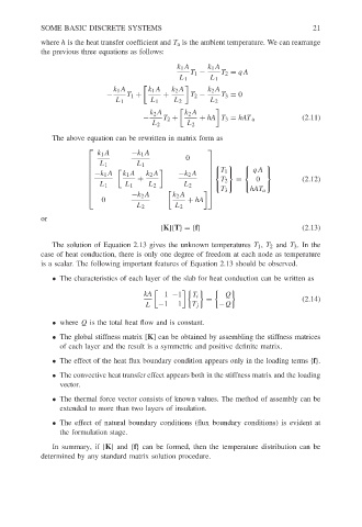
The above equation can be rewritten in matrix form as
k 1 A −k 1 A
 
0
L 1 L 1    
 
 
 −k 1 A k 1 A k 2 A −k 2 A  T 1  qA 
+ = 0 (2.12)
 
  T 2
 L 1 L 1 L 2 L 2     
 T 3 hAT a
−k 2 A k 2 A

 
0 + hA
L 2 L 2
or
[K]{T}={f} (2.13)
The solution of Equation 2.13 gives the unknown temperatures T 1 , T 2 and T 3 .Inthe
case of heat conduction, there is only one degree of freedom at each node as temperature
is a scalar. The following important features of Equation 2.13 should be observed.
• The characteristics of each layer of the slab for heat conduction can be written as
kA 1 −1 Q
T i
= (2.14)
L −1 1 T j −Q
• where Q is the total heat flow and is constant.

• The global stiffness matrix [K] can be obtained by assembling the stiffness matrices
of each layer and the result is a symmetric and positive definite matrix.

• The effect of the heat flux boundary condition appears only in the loading terms {f}.
• The convective heat transfer effect appears both in the stiffness matrix and the loading
vector.

• The thermal force vector consists of known values. The method of assembly can be
extended to more than two layers of insulation.

• The effect of natural boundary conditions (flux boundary conditions) is evident at
the formulation stage.

In summary, if [K]and {f} can be formed, then the temperature distribution can be
determined by any standard matrix solution procedure.