Page 31 - Fundamentals of The Finite Element Method for Heat and Fluid Flow

23
SOME BASIC DISCRETE SYSTEMS
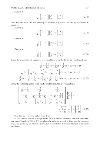
Element 1
1

1 −1
p 1
= q 1 (2.18)
−1 1
R 1 p 3 −q 1
Note that the mass flux rate entering an element is positive and leaving an element is
negative.
Element 2
1 1 −1 p 1 q 2
= (2.19)
−1 1
R 2 p 2 −q 2
Element 3
1 1 −1 p 2 q 3
= (2.20)
−1 1
R 3 p 3 −q 3
Element 4
1 1 −1 p 2 q 4
= (2.21)
−1 1
R 4 p 3 −q 4
From the above element equations, it is possible to write the following nodal equations:
1 1 1 1

+ p 1 − p 2 − p 3 = q 1 + q 2 = Q
R 1 R 2 R 2 R 1
1 1 1 1 1 1
− p 1 + + + p 2 − + p 3 = q 3 + q 4 − q 2 = 0
R 2 R 2 R 3 R 4 R 3 R 4
1 1 1 1 1 1
− p 1 − + p 2 + + + p 3 =−q 1 − q 3 − q 4 =−Q (2.22)
R 1 R 3 R 4 R 1 R 3 R 4
Now, the following matrix form can be written from the above equations:
 
1 1 1 1
+ − −
R 1 R 2 R 2 R 1  
 
 

1 1 1 1 1 1
  p 1
 
− + + − +  p 2 =

R 2 R 2 R 3 R 4 R 3 R 4
   
 p 3


1 1 1 1 1
 
1
− − + + +
R 1
R 3 R 4 R 1 R 3 R 4
   
q 1 + q 2
   Q 
−q 2 + q 3 + q 4 = 0 (2.23)
   
−q 1 − q 3 − q 4 −Q
Note that q 1 + q 2 = Q and q 2 = q 3 + q 4
In this fashion, we can solve problems such as electric networks, radiation networks,
and so on. Equations 2.18 to 2.21 are also valid and may be used to determine the pressures
if q 1 , q 2 , q 3 and q 4 are known a priori. Let us consider a numerical example to illustrate
the above.