Page 34 - Fundamentals of The Finite Element Method for Heat and Fluid Flow

26
j
i h, T a SOME BASIC DISCRETE SYSTEMS
k
Q i Q j

h, T a

L
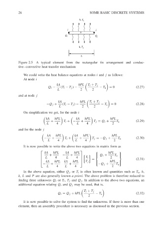
Figure 2.5 A typical element from the rectangular fin arrangement and conduc-
tive–convective heat transfer mechanism

We could write the heat balance equations at nodes i and j as follows:
At node i
kA hPL T i + T j
Q i − (T i − T j ) − − T a = 0 (2.27)
L 2 2
and at node j
kA hPL T i + T j
−Q j + (T i − T j ) − − T a = 0 (2.28)
L 2 2
On simplification we get, for the node i

kA hPL kA hPL hPL
+ T i + − + T j = Q i + T a (2.29)
L 4 L 4 2
and for the node j

kA hPL kA hPL hPL

− + T i + + T j =−Q j + T a (2.30)
L 4 L 4 2
It is now possible to write the above two equations in matrix form as
 
kA hPL kA hPL  hPL 
+ − +  Q i + 

 L 4 L 4  T i 2 T a 
  = (2.31)
 kA hPL kA hPL  T j  hPL 
− + +  −Q j + T a 
L 4 L 4 2
In the above equation, either Q j or T i is often known and quantities such as T a , h,
k, L and P are also generally known a priori. The above problem is therefore reduced to
finding three unknowns Q i or T i , T j and Q j . In addition to the above two equations, an
additional equation relating Q i and Q j may be used, that is,

T i + T j
Q i = Q j + hPL − T a (2.32)
2
It is now possible to solve the system to find the unknowns. If there is more than one
element, then an assembly procedure is necessary as discussed in the previous section.