Page 30 - Fundamentals of The Finite Element Method for Heat and Fluid Flow

22
1
q
1
3 SOME BASIC DISCRETE SYSTEMS
Q 1 q 3 Q
2 3
q 4
q 2 4
2
− Node
− Element
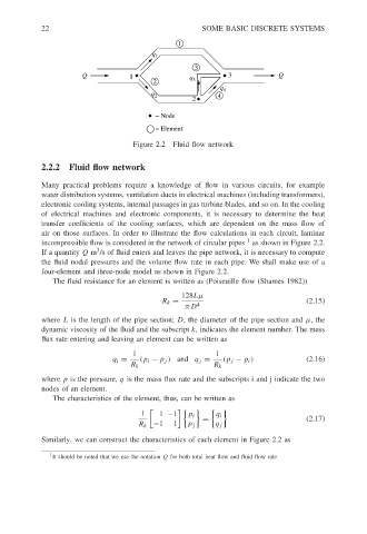
Figure 2.2 Fluid flow network

2.2.2 Fluid flow network

Many practical problems require a knowledge of flow in various circuits, for example
water distribution systems, ventilation ducts in electrical machines (including transformers),
electronic cooling systems, internal passages in gas turbine blades, and so on. In the cooling
of electrical machines and electronic components, it is necessary to determine the heat
transfer coefficients of the cooling surfaces, which are dependent on the mass flow of
air on those surfaces. In order to illustrate the flow calculations in each circuit, laminar
1
incompressible flow is considered in the network of circular pipes as shown in Figure 2.2.
3
If a quantity Q m /s of fluid enters and leaves the pipe network, it is necessary to compute
the fluid nodal pressures and the volume flow rate in each pipe. We shall make use of a
four-element and three-node model as shown in Figure 2.2.
The fluid resistance for an element is written as (Poiseuille flow (Shames 1982))
128Lµ
R k = (2.15)
πD 4
where L is the length of the pipe section; D, the diameter of the pipe section and µ,the
dynamic viscosity of the fluid and the subscript k, indicates the element number. The mass
flux rate entering and leaving an element can be written as

1 1
q i = (p i − p j ) and q j = (p j − p i ) (2.16)
R k R k
where p is the pressure, q is the mass flux rate and the subscripts i and j indicate the two
nodes of an element.
The characteristics of the element, thus, can be written as
1 1 −1 p i
q i
= (2.17)
R k −1 1 p j q j
Similarly, we can construct the characteristics of each element in Figure 2.2 as
1
It should be noted that we use the notation Q for both total heat flow and fluid flow rate