Page 115 - Fundamentals of Water Treatment Unit Processes : Physical, Chemical, and Biological

70 Fundamentals of Water Treatment Unit Processes: Physical, Chemical, and Biological

is selected when the finite difference solution approaches Example 4.1 Pulse Concentration Input
the mathematical solution, that is, when the ‘‘difference’’ to Complete Mix Reactor:
between the two solutions is small and the finite difference
solution is ‘‘stable,’’ meaning that the solution starts to 1. Statement: Determine C versus t for a complete mix
‘‘converge’’ as Dt decreases. reactor with the rate of reaction equal to zero, with
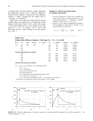
Table CD4.3 is an excerpt from Table CD4.2(b) showing constant flow and for C in ¼ 1000 mg=Lasa ‘‘pulse’’
function for the period, 0.1 t=u 0.5.
selected columns and enough rows to illustrate that a pulse
2. Solution scheme: Impose mathematical conditions
loading of salt occurs. Figure 4.13a is a plot of the output,
for the problem as stated, that is, [dC=dt] r ¼ 0, for
C t from Table CD4.2(b) for a pulse loading for the time
which Equation 4.34 becomes
period, 0.1 t=u 0.4. Figure 4.13b is a plot of the

same thing, but for a pulse loading for the time period, Q t
(C in, t C t ) Dt (Ex4:4:1)
0.1 t=u 1. C tþDt ¼ C t þ V
TABLE CD4.3
Solution Finite Difference Equation—Pulse Input (0.1 t=u 0.5) of Salt a
3
3
3
3
3
Dt (s) t (s) V (m ) Q (m =s) u ¼ V=Q (s) t=u C in,t (kg=m ) C t (kg=m ) C tþDt (kg=m )
0.01 0.00 1000 1000 1 0.00 100 100.000 100.000
0.01 0.01 100 100.000 100.000
0.02 0.02 100 100.000 100.000
0.03 0.03 100 100.000 100.000
* *
intentional discontinuity in spreadsheet
0.46 0.46 1000 373.228 379.496
0.47 0.47 1000 379.496 385.701
0.48 0.48 1000 385.701 391.844
0.49 0.49 1000 391.844 397.925
0.50 0.50 100 397.925 394.946
* *
intentional discontinuity in spreadsheet
Notes: (1) Dt is from ‘‘calibration’’ with mathematical solution.
(2) t ¼ t þ Dt.
(3) V is a design input.
(4) Q is the flow through the reactor.
(5) u is the detention time.
(6) C in is the specified salt concentration flowing into reactor.
(7) C t is the reactor concentration at, t Dt.
(8) C tþDt is the reactor concentration at time, t þ Dt, calculated by finite difference.
a
Printout of an excerpt from Table CD4.2 (b) for condition of ‘‘pulse’’ loading.

1000 1000
Salt pulse Salt pulse
Pulse inflow concentration is 1000 mg/L Pulse inflow concentration is 1000 mg/L
800 800
C =100 mg/L C =100 mg/L
i
i
600 600
C t C t
400 400
200 200

0 0
0 1 2 3 4 5 0 1 2 3 4 5
(a) t/θ (b) t/θ
FIGURE 4.13 Pulse flow displacement of solution in complete mix reactors plotted by Equation 4.34. (a) Pulse duration: t=u ¼ 0.4.
(b) Pulse duration: t=u ¼ 0.9.