Page 113 - Fundamentals of Water Treatment Unit Processes : Physical, Chemical, and Biological

68 Fundamentals of Water Treatment Unit Processes: Physical, Chemical, and Biological

1000 1000
900 900 C(initial) = 1000 mg/L
800 800
C(in)= 1000 mg/L=C when t/θ is large
700 700
C (mg/L) 600 C (mg/L) 600 C(in) =100 mg/L=C when t/θ is large
500
500
400
400
300 300
200 200
100 C(initial) = 100 mg/L 100
0 0
0 1 2 3 4 5 6 7 8 9 10 0 1 2 3 4 5 6 7 8 9 10
(a) t/θ (b) t/θ

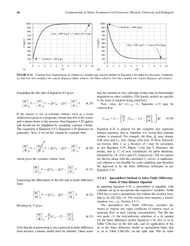
FIGURE 4.12 Constant flow displacement of solution in complete mix reactors plotted by Equation 4.28 under two boundary conditions.
(a) Salt flow into complete mix reactor displaces dilute solution. (b) Dilute solution flow into complete mix reactor displaces salt solution.

Expanding the left side of Equation 4.9 gives may be constant or vary with time or they may be functionally
dependent on other variables. [The kinetic models are specific
to the kind of situation being modeled.]
dC dV dC
V (4:29) Now, since DC ¼ C tþDt C t , Equation 4.33 may be
V þ
dt dt dt
C ¼ Q C in Q C
0 0 r
expressed as
If the reactor is not at constant volume, such as a waste ( )
stabilization pond in a temperate climate that fills in the winter Q t dC Dt (4:34)
C tþDt ¼ C t þ (C in, t C t )
and is drawn down in the summer, then Equation 4.29 applies V dt r, t
and should not be simplified by assuming constant volume.
The expansion of Equation 4.9 to Equation 4.29 illustrates its Equation 4.34 is general for the complete mix materials
generality. Now, if we let the volume be constant, then balance equation, that is, Equation 4.9, except that constant
volume is assumed. For example, the flow, Q, may change
with time and C in may change with time. If these functions
0
ƒƒ!
are known, then C as a function of t may be calculated,
dC dV dC V (4:30) as per Equation 4.34. Figure 4.12a and b illustrates the
dt V þ dt C ¼ Q C in Q C dt
0 0 r results, that is, C, of such calculations for pulse durations,
measured by t=u, of 0.4 and 0.9, respectively. The two pulses
which gives the constant volume form are shown, along with the calculated C t curves. A mathemat-
ical solution is not feasible for such conditions and therefore
the approach is by the finite difference technique, as per
dC dC
V (4:31) Equation 4.34.
V ¼ Q C in Q C
dt dt
0 r
4.3.4.5 Spreadsheet Method to Solve Finite Difference
Expressing the differential on the left side in finite difference Form of Mass Balance Equation
form
In applying Equation 4.34, a spreadsheet is required, with
columns set up to incorporate the respective variables. Table

DC dC
V (4:32) CD4.2(a) is such a spreadsheet, but without the reaction term,
V ¼ Q C in Q C
Dt dt
0 r that is, let [dC=dt] r ¼ 0. The reaction term requires a kinetic
equation (see, e.g., Section 4.4.1).
Dividing by V gives The spreadsheet file, Table CD4.2(a), provides the
means to impose any input conditions of interest (such as
unsteady flow or time varying concentration). The file has
DC Q dC
(4:33) two parts: (1) the trial-and-error selection of a Dt needed
¼
[C in C]
Dt V dt
0 r for the finite difference model, Equation 4.34, that is, as in
Table CD4.2(a) on the left side, and (2) application of the
Note that the reaction term is not expressed in finite difference Dt to the finite difference model in spreadsheet form, that
form because a kinetic model must be inserted. These terms is, as in Table CD4.2(b), on the right side. The Dt value