Page 116 - Fundamentals of Water Treatment Unit Processes : Physical, Chemical, and Biological

Unit Process Principles 71

3. Set up spreadsheet solution: The first step is to open Despite the aforementioned caveats, there are quite a few
the spreadsheet file, Table CD4.2(a). The second step things that we can say about kinetics. Some of the fundamen-
is to make a copy of the file to solve the problem at tals are reviewed.
hand. The copy with the required pulse loading
imposed is shown in the file as Table CD4.2(b) (cop-
ied side-by-side with Table CD4.2(a)). Table 4.3 is an 4.4.1 FIRST-ORDER KINETICS
excerpt of Table CD4.2(b). Figure 4.3 is a plot of the
The most widely used kinetic model is ‘‘first-order’’ that says
output, that is, t versus Ct from Table CD4.2(b), seen
simply that the rate of a given reaction for a disappearance of
also as in the copy, Table CD4.3.
a constituent, C, is proportional to the negative of the concen-
4. Discussion: To determine Dt in Equation E.4.1, a
tration at any instant and is expressed mathematically as
trial and error solution is required such that the
solution does not ‘‘blow up,’’ that is, become
unstable. Usually, picking successively smaller Dt dC ¼ kC (4:35)
values will soon result an appropriate value. But dt
then if a smaller Dt is used than is required, the
computing time becomes higher than necessary. in which
3
C is the concentration of a given constituent (kg=m )
For Equation 4.34, the boundary conditions may be t is the elapsed time from a given concentration, C 0 (s)
imposed such that solutions from the finite difference C 0 is the concentration of a given constituent at time, t ¼ 0
model and the mathematical model, Equation 4.28, are (kg=m )
3
about the same, for example, suppose a continuous k is the kinetic rate constant (s )
1
input of a salt solution at C in ¼ 1000 mg=L displaces a
C(reactor) ¼ 100 mg=L solution in the complete mix
reactor. Since the mathematical solution is exact, the effect Separation of the variables and integration gives
of choosing different Dt’s can be seen by comparing C t
values for each solution. In the spreadsheet file, Table ln C ¼ kt (4:36)
CD4.2(a), this may be evaluated by a column, ‘‘Diff,’’ that C 0
shows the difference between the two solutions. A suitable
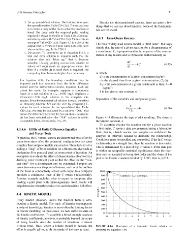
Dt has been selected when the ‘‘Diff’’ column is within Figure 4.14 illustrates the type of plot resulting. The slope is
acceptable limits, for example, 2%–3%. the kinetic constant, k.
To ascertain whether the reaction rate for a given reaction
4.3.4.6 Utility of Finite Difference Equation is first order, C versus t data are generated using a laboratory
flask, that is, a batch reactor, and samples are withdrawn for
and Tracer Tests
analyses at intervals needed to delineate the relationship.
In practice, the C versus t curves are determined most often by
Conditions must be specified and controlled. If the ln C versus
tracer tests since often the geometric configurations are more
t relationship is a straight line, then the reaction is first-order.
complex than simple complete mix reactor. These tests involve
This is determined by a plot of log C versus t. If the data plot
adding a ‘‘slug’’ of brine solution (or a fluorescent dye such as
is within an acceptable statistical significance, then the reac-
rhodamine-B or ponticyl pink) at some point of injection. An
tion may be accepted as being first order and the slope of the
example is to evaluate the effect of dispersion in a clear well in a
plot is the kinetic constant divided by 2.303, that is, k=2.3.
drinking water treatment plant so that the effect on the ‘‘con-
tact-time’’ for a disinfectant can be evaluated. Samples are
taken downstream at the point of interest, such as at the outflow
of the basin (a conductivity sensor with output to a computer 1000
provides a continuous trace of the C versus t relationship). 900 C(initial)= C = 1000 mg/L
0
Another example includes what to expect in sampling after 800
seeding a pilot plant with microorganisms. Such results will
700
help determine when the seed arrives and when it has full effect. 600
C (mg/L) 500
4.4 KINETIC MODELS 400
Every reactor situation, unless the reaction term is zero, 300
requires a kinetic model. The topic of kinetics encompasses 200
a body of knowledge; kinetics is most often the limiting factor
100
in reactor modeling. In most cases, we lack sufficient data on
0
the kinetic coefficients. To establish a broad enough database
0 1 2 3 4 5 6 7 8 9 10
of kinetic coefficients, however, is probably beyond the scope
t
of being feasible since the number of situations is almost
without limit. Thus, where a kinetic model is needed, the FIGURE 4.14 Illustration of a first-order kinetic relation as
effort is usually ad hoc to fit the needs of the case at hand. described by Equation 4.36.