Page 112 - Fundamentals of Water Treatment Unit Processes : Physical, Chemical, and Biological

Unit Process Principles 67

∂(C·V) 1.0
∂t 0.9
obs
0.8
Reactor 0.7
0 0.6 (–t/θ)
Q·C in Q·C (C– C in )/(C i –C in ) 0.5 e
∂(C·V)
∂t 0.4
r 0.3
0.2
FIGURE 4.10 Steady state materials balance for a batch reactor,
0.1
that is, for a complete mix reactor when the observed rate of reaction
0.0
is zero.
0 1 2 3 4 5 6 7 8 9 10
t/θ
time) increases. All that remains in this case is to apply a
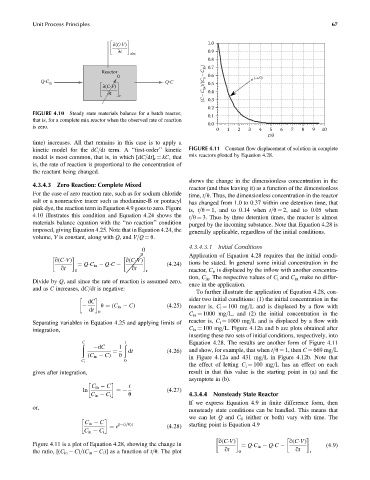
kinetic model for the dC=dt term. A ‘‘first-order’’ kinetic FIGURE 4.11 Constant flow displacement of solution in complete
model is most common, that is, in which [dC=dt] r ¼ kC, that mix reactors plotted by Equation 4.28.
is, the rate of reaction is proportional to the concentration of
the reactant being changed.
shows the change in the dimensionless concentration in the
4.3.4.3 Zero Reaction: Complete Mixed
reactor (and thus leaving it) as a function of the dimensionless
For the case of zero reaction rate, such as for sodium chloride time, t=u. Thus, the dimensionless concentration in the reactor
salt or a nonreactive tracer such as rhodamine-B or pontacyl has changed from 1.0 to 0.37 within one detention time, that
pink dye, the reaction term in Equation 4.9 goes to zero. Figure is, t=u ¼ 1, and to 0.14 when t=u ¼ 2, and to 0.05 when
4.10 illustrates this condition and Equation 4.24 shows the t=u ¼ 3. Thus by three detention times, the reactor is almost
materials balance equation with the ‘‘no reaction’’ condition purged by the incoming substance. Note that Equation 4.28 is
imposed, giving Equation 4.25. Note that in Equation 4.24, the generally applicable, regardless of the initial conditions.
volume, V is constant, along with Q, and V=Q ¼ u.
4.3.4.3.1 Initial Conditions
0
ƒƒƒ!
Application of Equation 4.28 requires that the initial condi-
q(C V) q(C V) (4:24) tions be stated. In general some initial concentration in the
qt ¼ Q C in Q C qt
0 r reactor, C i , is displaced by the inflow with another concentra-
tion, C in . The respective values of C i and C in make no differ-
Divide by Q, and since the rate of reaction is assumed zero,
ence in the application.
and as C increases, dC=dt is negative:
To further illustrate the application of Equation 4.28, con-
sider two initial conditions: (1) the initial concentration in the
dC
u ¼ (C in C) (4:25) reactor is, C i ¼ 100 mg=L and is displaced by a flow with
dt

0 C in ¼ 1000 mg=L, and (2) the initial concentration in the
Separating variables in Equation 4.25 and applying limits of reactor is, C i ¼ 1000 mg=L and is displaced by a flow with
integration, C in ¼ 100 mg=L. Figure 4.12a and b are plots obtained after
inserting these two sets of initial conditions, respectively, into
ð C ð t Equation 4.28. The results are another form of Figure 4.11
dC 1
dt (4:26) and show, for example, that when t=u ¼ 1, then C ¼ 669 mg=L
(C in C) u in Figure 4.12a and 431 mg=L in Figure 4.12b. Note that
¼
C i 0
the effect of letting C i ¼ 100 mg=L has an effect on each
gives after integration, result in that this value is the starting point in (a) and the
asymptote in (b).

C in C t
ln ¼ (4:27)
C in C i u 4.3.4.4 Nonsteady State Reactor
If we express Equation 4.9 in finite difference form, then
or,
nonsteady state conditions can be handled. This means that
we can let Q and C 0 (either or both) vary with time. The

C in C [ (t=u)]
¼ e (4:28) starting point is Equation 4.9
C in C i

q(C V) q(C V)
Figure 4.11 is a plot of Equation 4.28, showing the change in (4:9)
¼ Q C in Q C
the ratio, [(C in C)=(C in C i )] as a function of t=u. The plot qt 0 qt r