Page 183 - Fundamentals of Water Treatment Unit Processes : Physical, Chemical, and Biological

138 Fundamentals of Water Treatment Unit Processes: Physical, Chemical, and Biological

1.2 where
1.1 x is the horizontal distance from vertical center line to point
on curved edge of weir (m)
1
y is the vertical distance from the base of the curve, at
0.9
height a, to same point on curved edge of weir (m)
0.8
b is the width of half of the rectangular base part of
0.7 weir (m)
y 0.6 a is the height of rectangular base part of weir (m)
Q (half-section) is the flow through half of the weir section,
0.5
that is, either the half to the right or the half to the left of
0.4 3
the vertical center-line (m =s)
2
0.3 K is the coefficient for weir (m =s)
0.2 h is the depth of water from bottom of rectangular base to
water surface (m)
0.1
C is the discharge coefficient, which is taken as 1.0 in the
0 literature (dimensionless)
x (m) 2
g is the acceleration of gravity (9.81 m=s )
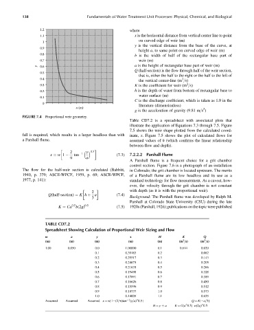
FIGURE 7.4 Proportional weir geometry.
Table CD7.2 is a spreadsheet with associated plots that
illustrate the application of Equations 7.3 through 7.5. Figure
7.5 shows the weir shape plotted from the calculated coord-
fall is required, which results in a larger headloss than with inate, x. Figure 7.5 shows the plot of calculated flows for
a Parshall flume. assumed values of h (which confirms the linear relationship
between flow and depth).

2 1
y 0:5
tan (7:3) 7.2.2.2 Parshall Flume
x ¼ w 1
p a
A Parshall flume is a frequent choice for a grit chamber
control section. Figure 7.6 is a photograph of an installation
The flow for the half-weir section is calculated (Babbitt, in Colorado; the grit chamber is located upstream. The merits
1940, p. 379; ASCE-WPCF, 1959, p. 69; ASCE-WPCF, of a Parshall flume are its low headloss and its use as a
1977, p. 141): standard technology for flow measurement. As a caveat, how-
ever, the velocity through the grit chamber is not constant
with depth (as it is with the proportional weir).
2
Q(half-section) ¼ Kh þ a (7:4)
3 Background: The Parshall flume was developed by Ralph M.
Parshall at Colorado State University (CSU) during the late
0:5 0:5
K ¼ Ca b(2g) (7:5) 1920s (Parshall, 1926); publications on the topic were published

TABLE CD7.2
Spreadsheet Showing Calculation of Proportional Weir Sizing and Flow
w a y x H K Q
3
2
(m) (m) (m) (m) (m) (m =s) (m =s)
1.00 0.050 0.0 1.00000 0.1 0.614 0.020
0.1 0.39183 0.2 0.082
0.2 0.29517 0.3 0.143
0.3 0.24675 0.4 0.205
0.4 0.21635 0.5 0.266
0.5 0.19498 0.6 0.328
0.6 0.17891 0.7 0.389
0.7 0.16626 0.8 0.450
0.8 0.15596 0.9 0.512
0.9 0.14737 1.0 0.573
1.0 0.14005 1.1 0.635
1
Assumed Assumed Assumed x ¼ w[1 (2=p)tan (y=a) 0.5] Q ¼ K[ a=3]
^
H ¼ y þ a K ¼ C(a 0.5) w(2g) 0.5
^
^