Page 309 - Fundamentals of Water Treatment Unit Processes : Physical, Chemical, and Biological

264 Fundamentals of Water Treatment Unit Processes: Physical, Chemical, and Biological

10.4.1.2.2 Derivation of Blend Number C in C [ t=u]
¼ e (10:36)
While the ‘‘blend number’’ appears to be empirical, a rationale C in C i
may be seen, as given in the account following.
where
From Equation 10.35, i.e., t 5R 5 u(impeller), substitute C in is the concentration of substance A in flow entering
3
q(impeller) ¼ V(reactor)=Q(impeller), reactor at any time, t 0 (kg=m )
2
where V(reactor) ¼ pT H=4 and Q(impeller) ¼ QnD C i is the initial concentration of substance A in reactor, i.e.,
3
3
(impeller) , then collect the numerical terms, let H ¼ T, and at t ¼ 0 (kg=m )
move n to the left side, to give, n(impeller) t 5R ¼ (35.34=Q). C is the concentration of substance A in reactor at any
3
Then, from Table 10.6, time, t (kg=m )
K(0.99 blend, Rushton system) 36, t is the elapsed time after start of substance A in flow to
reactor (s)
which gives Q 0.98, which is larger than the accepted range
0.54 Q 0.88 for the Rushton 6-blade impeller. While u(reactor) is the detention time of reactor, i.e., u(reactor) ¼
Q=V (s)
Q 0.98 is higher than ‘‘hoped-for,’’ the rationale to obtain it
is logical and the discrepancy is not large.
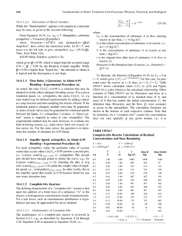
To illustrate, the behavior of Equation 10.36, let C in ¼ 0at
t > 0, which gives C=C i ¼ e ( t=u(reactor)) . For this case, let pure
10.4.1.3 Time Ratio, t=Q(reactor), to Attain 0.99
water enter the reactor at t > 0; thus, at t ¼ 0, C ¼ C i . Table
Blending—Experimental Procedure (a)
CD10.7 shows calculated values C=C i vs. (t=u) and Figure
As noted, the ratio C(t)=C o 0.99 is a criterion that may be CD10.18 is a plot linked to the calculated relationship. Other
adopted to define when adequate blending occurs. For a given columns of Table CD10.7 are for illustration and show as a
rotational speed, i.e., w(impeller), the curve C(t)=C o vs. t=q function of t: concentration of A, residual mass of A, and
(raw water) may be defined experimentally by adding a tracer mass of A that has exited; the initial concentration, C i , the
as a step function and then sampling the reactor effluent. If the detention time, u(reactor), and the flow, Q, were assumed,
rotational speed is changed, another curve may be generated. as given in the spreadsheet. The calculation formulae are
A series of such curves may be generated for rotational speeds shown at the bottom of each respective column. Note that
between the limits, 0 w(impeller) w(max). A ‘‘direct-cur- by definition, for a ‘‘complete-mix’’ reactor the concentration
rent’’ motor is required in order to vary w(impeller). The does not vary spatially at any given instant, i.e., it is
experimental method may be used, however, to evaluate any
kind of mixing system, e.g., static mixer, back-mix reactor, in-
line mixer, etc. For the static mixer, the question is to deter-
TABLE CD10.7
mine the number of elements for 0.99 blend.
Complete-Mix Reactor Calculations of Residual
Concentrations and Mass Remaining
10.4.1.4 Impeller Speed, w(impeller), to Attain 0.99
Blending—Experimental Procedure (b) u ¼ 10 s V ¼ 1.000 m 3
3
3 Q ¼ 0.100 m =s
C i ¼ 1000 kg=m
For each w(impeller) value, the particular value of t=q(raw
water) that occurs when C(t)=C o 0.99 permits a second plot, C t C Mass R Mass Exited
3
i.e., [t=q(raw water)] C(t)C o 0.99 vs. w(impeller). The second t=q C i (s) (kg=m ) (kg) (kg)
plot should have enough points to define the curve, e.g., for 0.0 1.00 0.00 1000 1000 0.00
[t=q(raw water)] C(t)C o 0.99 >> 1.0. Entering the plot at [t=q 0.1 0.90 1.00 905 905 95
(raw water)] C(t)C o 0.99 1.0 yields the sought value of impel- 0.2 0.82 2.00 819 819 181
ler speed, i.e., [w(impeller)] C(t)C o 0.99 . In other words, this is 0.3 0.74 3.00 741 741 259
the impeller speed that results in 0.99-fraction blend for one 0.4 0.67 4.00 670 670 330
raw-water detention time. 0.5 0.61 5.00 607 607 393
0.6 0.55 6.00 549 549 451
10.4.1.5 Complete-Mix Reactors 0.7 0.50 7.00 497 497 503
0.8 0.45 8.00 449 449 551
The defining characteristic of a ‘‘complete-mix’’ reactor is that
0.9 0.41 9.00 407 407 593
upon the addition of a finite mass of a substance ‘‘A’’ to the
1.0 0.37 10.00 368 368 632
reactor, a homogeneous concentration results instantaneously.
1.5 0.22 15.00 223 223 777
For a real mixer, such an instantaneous distribution is hypo-
2.0 0.14 20.00 135 135 865
thetical and may be approached but never attained.
3.0 0.05 30.00 50 50 950
4.0 0.02 40.00 18 18 982
10.4.1.5.1 Mathematics of Complete-Mix 5.0 0.01 50.00 7 7 993
The mathematics of a complete-mix reactor is reviewed in
¼ exp( t=q) ¼ (C=C i ) C i ¼ [C i C]
Section 4.3.3, e.g., as described by Equations 4.24 through
¼ (t=q) q ¼ C V(reactor) V(reactor)
4.28. Equation 4.28 is repeated as Equation 10.36, i.e.,