Page 521 - Fundamentals of Water Treatment Unit Processes : Physical, Chemical, and Biological

476 Fundamentals of Water Treatment Unit Processes: Physical, Chemical, and Biological

–
ΔX – –
Particle kinetics: = D C (X*–X)
s
1.0 Δt
P
Inflection point: (C΄, Z΄)
0
0
C/C 0 –
–
1
P
Advection kinetics: ΔX = (v+ Dλ) λC
Δt ρ 1– P
A
C –λ(Z– Z΄)
= e 0
C 0
0
Z
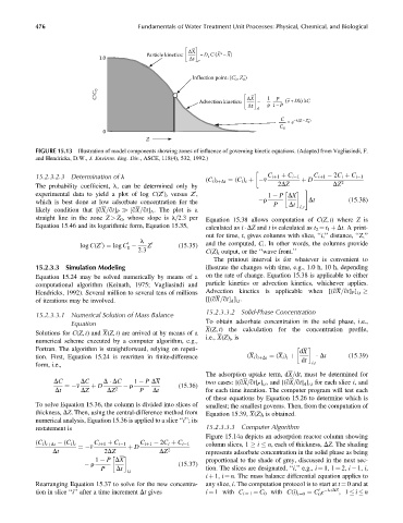
FIGURE 15.13 Illustration of model components showing zones of influence of governing kinetic equations. (Adapted from Vagliasindi, F.
and Hendricks, D.W., J. Environ. Eng. Div., ASCE, 118(4), 532, 1992.)

15.2.3.2.3 Determination of l C iþ1 þ C i 1 C iþ1 2C i þ C i 1
(C i ) tþDt ¼ (C i ) t þ v þ D 2
The probability coefficient, l, can be determined only by 2DZ DZ
#

experimental data to yield a plot of log C(Z ) t versus Z , 1 P DX
0
0
which is best done at low adsorbate concentration for the r P Dt Dt (15:38)
likely condition that [qX=qt] P [qX=qt] A . The plot is a i, t
straight line in the zone Z > Z 0 , whose slope is l=2.3 per Equation 15.38 allows computation of C(Z, t) where Z is
Equation 15.46 and its logarithmic form, Equation 15.35, calculated as i DZ and t is calculated as t 2 ¼ t 1 þ Dt. A print-
out for time, t, gives columns with slice, ‘‘i,’’ distance, ‘‘Z,’’
l
0 0 Z 0 (15:35) and the computed, C i . In other words, the columns provide
0
2:3 C(Z) t output, or the ‘‘wave front.’’
log C(Z ) ¼ log C
The printout interval is for whatever is convenient to
15.2.3.3 Simulation Modeling illustrate the changes with time, e.g., 1.0 h, 10 h, depending
Equation 15.24 may be solved numerically by means of a on the rate of change. Equation 15.38 is applicable to either
computational algorithm (Keinath, 1975; Vagliasindi and particle kinetics or advection kinetics, whichever applies.
Hendricks, 1992). Several million to several tens of millions Advection kinetics is applicable when [(qX=qt] P ] i,t
of iterations may be involved. [[(qX=qt] A ] i,t .
15.2.3.3.2 Solid-Phase Concentration
15.2.3.3.1 Numerical Solution of Mass Balance
Equation To obtain adsorbate concentration in the solid phase, i.e.,
X(Z, t) the calculation for the concentration profile,
Solutions for C(Z, t) and X(Z, t) are arrived at by means of a
i.e., X(Z) t ,is
numerical scheme executed by a computer algorithm, e.g.,
Fortran. The algorithm is straightforward, relying on repeti-
dX
tion. First, Equation 15.24 is rewritten in finite-difference (X i ) tþDt ¼ (X i ) t þ Dt (15:39)
dt i,t
form, i.e.,
The adsorption uptake term, dX=dt, must be determined for
DC DC D DC 1 P DX two cases: [(qX=qt] P ] i,t , and [(qX=qt] A ] i,t for each slice i, and
¼ v þ D r (15:36)
Dt DZ DZ 2 P Dt for each time iteration. The computer program will test each
of these equations by Equation 15.26 to determine which is
To solve Equation 15.36, the column is divided into slices of smallest; the smallest governs. Then, from the computation of
thickness, DZ. Then, using the central-difference method from Equation 15.39, X(Z) t is obtained.
numerical analysis, Equation 15.36 is applied to a slice ‘‘i’’; its
restatement is 15.2.3.3.3 Computer Algorithm
Figure 15.14a depicts an adsorption reactor column showing
(C i ) tþDt (C i ) t C iþ1 þ C i 1 C iþ1 2C i þ C i 1 column slices, 1 i n, each of thickness, DZ. The shading
¼ v þ D
Dt 2DZ DZ 2 represents adsorbate concentration in the solid phase as being

1 P DX proportional to the shade of grey, discussed in the next sec-
r (15:37)
P Dt tion. The slices are designated, ‘‘i,’’ e.g., i ¼ 1, 1 ¼ 2, i 1, i,
i,t
i þ 1, i ¼ n. The mass balance differential equation applies to
Rearranging Equation 15.37 to solve for the new concentra- any slice, i. The computation protocol is to start at t ¼ 0andat
0 l iDZ
tion in slice ‘‘i’’ after a time increment Dt gives i ¼ 1 with C i ¼ 1 ¼ C 0 with C(i) t¼0 ¼ C e ,1 i n
0