Page 522 - Fundamentals of Water Treatment Unit Processes : Physical, Chemical, and Biological

Adsorption 477

Q C 0

i =1
i=2
0 C C 0
0

C(Z) t =0
Saturated zone at time, t
Z
i –1 Z o ΄
i Δz
i +1

C 0 ΄
C(Z) t
C(Z) t+Δt
Inflection point
i = n

(a) QC (b)
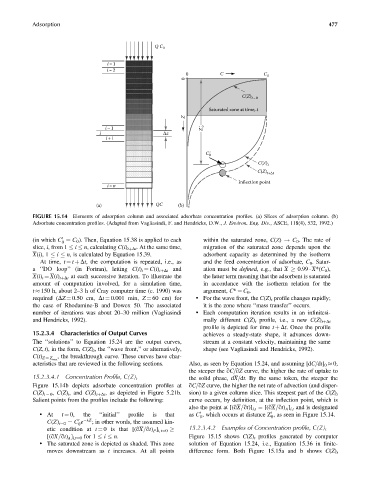
FIGURE 15.14 Elements of adsorption column and associated adsorbate concentration profiles. (a) Slices of adsorption column. (b)
Adsorbate concentration profiles. (Adapted from Vagliasindi, F. and Hendricks, D.W., J. Environ. Eng. Div., ASCE, 118(4), 532, 1992.)

(in which C ¼ C 0 ). Then, Equation 15.38 is applied to each within the saturated zone, C(Z) ! C 0 . The rate of
0
0
slice, i, from 1 i n, calculating C(i) tþDt . At the same time, migration of the saturated zone depends upon the
X(i), 1 i n, is calculated by Equation 15.39. adsorbent capacity as determined by the isotherm
At time, t ¼ t þ Dt, the computation is repeated, i.e., as and the feed concentration of adsorbate, C 0 . Satur-
a ‘‘DO loop’’ (in Fortran), letting C(i) t ¼ C(i) tþDt and ation must be defined, e.g., that X 0.99 X*(C 0 ),
X(i) t ¼ X(i) tþDt at each successive iteration. To illustrate the the latter term meaning that the adsorbent is saturated
amount of computation involved, for a simulation time, in accordance with the isotherm relation for the
t 150 h, about 2–3 h of Cray computer time (c. 1990) was argument, C* ¼ C 0 .
required (DZ ¼ 0.50 cm, Dt ¼ 0.001 min, Z ¼ 60 cm) for . For the wave front, the C(Z) t profile changes rapidly;
the case of Rhodamine-B and Dowex 50. The associated it is the zone where ‘‘mass transfer’’ occurs.
number of iterations was about 20–30 million (Vagliasindi . Each computation iteration results in an infinitesi-
and Hendricks, 1992). mally different C(Z) t profile, i.e., a new C(Z) tþDt
profile is depicted for time t þ Dt. Once the profile
15.2.3.4 Characteristics of Output Curves achieves a steady-state shape, it advances down-
The ‘‘solutions’’ to Equation 15.24 are the output curves, stream at a constant velocity, maintaining the same
C(Z, t), in the form, C(Z) t , the ‘‘wave front,’’ or alternatively, shape (see Vagliasindi and Hendricks, 1992).
, the breakthrough curve. These curves have char-
C(t) Z ¼ Z max
acteristics that are reviewed in the following sections. Also, as seen by Equation 15.24, and assuming [dC=dt] 0 0,
the steeper the qC=qZ curve, the higher the rate of uptake to
15.2.3.4.1 Concentration Profile, C(Z) t the solid phase, dX=dt. By the same token, the steeper the
Figure 15.14b depicts adsorbate concentration profiles at qC=qZ curve, the higher the net rate of advection (and disper-
C(Z) t ¼ 0 , C(Z) t , and C(Z) tþDt , as depicted in Figure 5.21b. sion) to a given column slice. This steepest part of the C(Z) t
Salient points from the profiles include the following: curve occurs, by definition, at the inflection point, which is
also the point at [(qX=qt)] i,t ¼ [(qX=qt) ] i,t and is designated
A
. At t ¼ 0, the ‘‘initial’’ profile is that as C , which occurs at distance Z , as seen in Figure 15.14.
0
0
0 0
0 lZ
C(Z) t¼0 ¼ C e ; in other words, the assumed kin-
0
15.2.3.4.2 Examples of Concentration profile, C(Z) t
etic condition at t ¼ 0 is that [(qX=qt) P ] i, t¼0
[(qX=qt) A ] i,t¼0 for 1 i n. Figure 15.15 shows C(Z) t profiles generated by computer
. The saturated zone is depicted as shaded. This zone solution of Equation 15.24, i.e., Equation 15.36 in finite-
moves downstream as t increases. At all points difference form. Both Figure 15.15a and b shows C(Z) t