Page 524 - Fundamentals of Water Treatment Unit Processes : Physical, Chemical, and Biological

Adsorption 479

breakthrough curve for Run #QUPR is seen to emerge at
about t 32 h with midpoint at about t 39 h. BOX 15.3 MODELING: MATHEMATICAL
The breakthrough curve may, in fact, be ‘‘mapped’’ from VERSUS PHYSICAL
the wave front, i.e., by the chain rule (see any text on differ-
Mathematical modeling of packed-bed reactors has not
ential equations), i.e.,
been applied often (i.e., directly to design) for several
dC qC qZ reasons: (1) the variables in the model—especially the
(15:40) kinetic ones—require extensive laboratory testing to
¼
dt qZ qt

determine; (2) the model must be in the form of a
and, for a given position on the wave front, computer algorithm to execute, e.g., Fortran; (3) a
high-speed computer is required to run the program;
qZ (4) the model is complex. The main limiting factor,
(15:41)
qt however, is the extensive laboratory effort required to
v wf ¼
generate the needed kinetic coefficients and then to
where v wf is the velocity of wave front (m=s).
analyze the results. A final limitation, that warrants
Therefore,
special mention, is that the general model described is
for a single adsorbate, whereas most real situations
dC qC
(15:42) involve a mixture of adsorbates.
dt qZ
¼ v wf
A physical model, i.e., a pilot plant, essentially
Equation 15.42 shows the relationship between the break- ‘‘short circuits’’ the difficulties of mathematical model-
and the wave front, C(Z) t ; from ing by empirically ‘‘integrating’’ the effects of inde-
through curve, C(t) Z ¼ Z max
this the breakthrough curve for Run #QUPR, shown in pendent variables in terms of C(Z) t profiles or,
Figure 15.16b, may be mapped from the wave front, shown alternatively, of ‘‘breakthrough’’ curves, i.e., C(t) Z ¼ Z max .
in Figure 15.16a. In other words, the emergence of the wave In addition, the physical model may incorporate vari-
front from the column defines the breakthrough curve (see, for ables that were not anticipated in mathematical model-
example, Vagliasindi and Hendricks, 1992). ing. Biological growths are an example of the latter.
i.e., the extent and the effect of biological growth.
15.2.3.4.4 Solid-Phase Adsorbate Concentration Competitive effects, e.g., of two or more adsorbates or
background organic matter, are integrated as well. Two
Profile, X(Z) t
Uptake to the solid phase is given as scales of physical models are (1) pilot plant, and
(2) demonstration (discussed in subsequent sections).
Due to slow particle uptake rate in some situations,
dX
Dt (15:43) physical modeling could require several weeks or
dt
X Z,rþDt ¼ X Z, t þ
Z, t months of operation.
While not practical for direct application in design or
which is the same as Equation 15.39. As the adsorbent
operation, a mathematical model has other kinds of
becomes ‘‘saturated’’ with adsorbent at the higher levels of
utility: (1) scenarios may be imposed to examine the
the column, the solid-phase ‘‘wave front’’ translates down-
trends caused by different variables; (2) the model helps
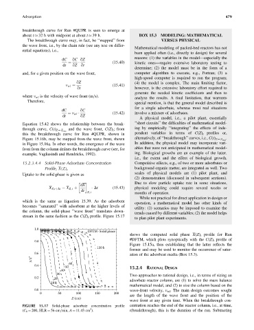
stream in the same fashion as the C(Z) t profile. Figure 15.17
to plan pilot plant experiments.
1.0
DFTM-Solid phase
shows the computed solid phase X(Z) t profile for Run
#DFTM, which plots synoptically with the C(Z) t profile of
0.8
Figure 15.15a, thus establishing that the latter reflects the
130 h
former and may be used to monitor the occurrence of satur-
0.6 ation of the adsorbent media (Box 15.3).
χ/χ*
0.4 50 60
40 15.2.4 RATIONAL DESIGN
30 Two approaches to rational design, i.e., in terms of sizing an
0.2 20
10 h adsorbate reactor column, are (1) to solve the mass balance
mathematical model, and (2) to size the column based on the
0.0 wave-front velocity, v wf . The main design outcomes sought
0 50 100 150 200
are the length of the wave front and the position of the
Z (cm)
wave front at any given time. When the breakthrough con-
FIGURE 15.17 Solid-phase adsorbate concentration profile centration reaches the end of the reactor column, i.e., at time,
2
(C 0 ¼ 200, HLR ¼ 56 cm=min, A ¼ 11.43 cm ). t(breakthrough), this is the duration of the run. Subtracting