Page 868 - Fundamentals of Water Treatment Unit Processes : Physical, Chemical, and Biological

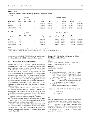
Appendix E: Porous Media Hydraulics 823

TABLE CDE.2
Conversion between K and k Including Headloss Calculation from k
(a) K to k
g ¼ 9.807 Enter K to Calculate k
K K T k
d 10 d 60 d 50 m r w
3
2
2
Media Name (mm) (mm) (mm) UC (m=d) (m=s) (8C) (Ns=m ) (kg=m ) (m )
Sand 0.50 1.5 2.42Eþ02 2.80E 03 3 0.00162 999.965 4.622E 10
Anthracite 0.91 1.5 1.26Eþ03 1.46E 02 3 0.00162 999.965 2.419E 09
Flatiron masonry 0.24 2.7 3.77Eþ01 4.37E 04 3 0.00162 999.965 7.215E 11
Flatiron masonry 0.24 2.7 4.08Eþ01 4.72E 04 3 0.00162 999.965 7.804E 11
(b) k to K
g ¼ 9.807 Enter k to Calculate K

d 10 d 60 d 50 k T m r w K K
2
3
2
Media Name (mm) (mm) (mm) UC (m ) (8C) (Ns=m ) (kg=m ) (m=s) (m=d)
Sand 0.50 1.5 4.62E 10 3 0.00162 999.965 2.80E 03 2.4162Eþ02
Anthracite 0.91 1.5 2.42E 09 3 0.00162 999.965 1.46E 02 1.2644Eþ03
Flatiron masonry 0.24 2.7 7.21E 11 3 0.00162 999.965 4.37E 04 3.7717Eþ01
Flatiron masonry 0.24 2.7 7.80E 11 3 0.00162 999.965 4.72E 04 4.0800Eþ01
Notes:
2
3
m(water) ¼ 0.00178024 5.61324 10 05 T þ 1.003 10 06 T 7.541 10 09 T .
4
5
2
3
r(water) ¼ 999.84 þ 0.068256 T – 0.009144 T þ 0.00010295 T – 1.1888 10 06 T þ 7.1515 10 09 T .
conditions, e.g., as in Table CDE.2(b). From K, headloss may Example E.1 Calculation of Headloss for Given
be calculated for a given HLR value and column length. Conditions of Filter Media
Given
E.3.4 PERMEABILITY DATA FOR FILTER MEDIA
d 10 ¼ 1.5 mm anthracite, P ¼ 0.45, v ¼ 18 m=h (7.4
2
As noted, the h L =Dz versus v data of Chang et al. (1999) for gpm=ft ), media depth ¼ 2.0 m, T ¼ 208C
30 tests were for 3 sand sizes, 3 anthracite sizes and 1.5 mm Required
glass beads, and with 3 or more porosity levels for each Headloss, i.e., clean bed
media. Porosity was controlled, as feasible, by tapping on
Solution
the 101 mm (4 in.) columns or by varying the rate
1. Determine k: From Figure E.3, for d 10 ¼ 1.5 mm and
of backwash termination. As noted, Figure E.1b characterized 9 2
P ¼ 0.45, k 4.0 10 m . Comparing this with the
the trends found in each plot. The linear portion of a given k versus P plot of Figure E.2, adjust k upward slightly
plot was used to estimate the hydraulic conductivity, i.e., to give, k 4.5 10 9 m .
2
1=slope ¼ K. The data also stated the temperature of each 2. Determine R: R ¼ rvd 10 =m ¼ 998 0.005 (1.5=1000)=
test which permitted the calculation of intrinsic permeability, 0.001¼ 7.5, which is at the approximate upper limit
k, by Equation E.5. As noted, the k is a characteristic of the for the application of the Darcy equation.
media and so it has more utility than K (since temperature 3. Apply Darcy’s equation: Equation E.5 is the form
affects the latter). applied and with numerical data substituted,
Figures E.2 and E.3 show plots of k versus P and k versus
0:005 m=s ¼ 4:5 10 9
d 10 , respectively, derived from the Chang, et al. (1999) h L =Dz 998 9:81=0:001Þ h L =2:0Þ
ð
ð
versus v data. The ‘‘groups’’ seen in Figure E.2 are for tests ¼ 0:0220 h L
with different sands as characterized by their d 10 values.
h L ¼ 0:227 m
A linear trend of k versus P is seen for each group.
Figure E.3 shows the same data but plotted as k versus d 10 ,
Discussion
and grouped by porosity; the two CSU data points are from
First, the estimate of clean-bed headloss is reasonable,
Hendricks et al. (1991). An approximate envelope is shown
based upon experience. Second, although the plots, i.e.,
for the data by the two lines (upper and lower).
Figures E.2 and E.3 are not definitive, the trend in Figure
From the k data, taken from either Figure E.2 or E.3, head
E.3, i.e., k versus d 10 for the loci of constant’s, seems
loss may be calculated based on for any assumed set of design consistent. Third, there should be some estimate of uncer-
conditions, e.g., T, DZ, HLR. Note that any selection of k tainty. If the porosity, P, was not stated, we would most
2
involves uncertainty, as suggested by the envelope of data likely state that 2 10 9 < k < 4 10 9 m which would
seen in Figure E.3. give, 100 < h L < 200 mm.