Page 875 - Fundamentals of Water Treatment Unit Processes : Physical, Chemical, and Biological

830 Appendix E: Porous Media Hydraulics

Forchheimer equation becomes the Darcy equation. The
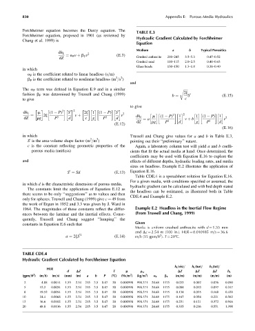
TABLE E.3
Forchheimer equation, proposed in 1901 (as reviewed by
Hydraulic Gradient Calculated by Forchheimer
Chang et al. 1999) is
Equation
Medium a b Typical Porosities
dh L 2
¼ a F v þ b v (E:3)
F
dZ Crushed anthracite 210–245 3.5–5.3 0.47–0.52
Crushed sand 110–115 2.0–2.5 0.40–0.43
Glass beads 130–150 1.3–1.8 0.38–0.40
in which
a F is the coefficient related to linear headloss (s=m)
2
2
b F is the coefficient related to nonlinear headloss (m =s )
and
The a F term was defined in Equation E.9 and in a similar r ffiffiffiffiffi
2j
fashion b F was determined by Trussell and Chang (1999) S 0 (E:15)
b ¼
to give c
to give
2
0 2
dh L m (1 P) S 2j 1 (1 P) S 0 2
2j v þ v m (1 P) 2 1 2 1 (1 P) 1
¼
dZ rg P 3 d c g P 3 d dh L ¼ a v þ b v 2
dZ rg P 3 d g P 3 d
(E:12)
(E:16)
in which Trussell and Chang give values for a and b in Table E.3,
2 3
S is the area-volume shape factor (m =m ) pointing out their ‘‘preliminary’’ nature.
0
c is the constant reflecting geometric properties of the Again, a laboratory column test will yield a and b coeffi-
porous media (unitless) cients that fit the actual media at hand. Once determined, the
coefficients may be used with Equation E.16 to explore the
and effects of different depths, hydraulic loading rates, and media
sizes on headloss. Example E.2 illustrates the application of
S ¼ Sd (E:13) Equation E.16.
0
Table CDE.4 is a spreadsheet solution for Equation E.16.
For a given media, with conditions specified or assumed, the
in which d is the characteristic dimension of porous media.
hydraulic gradient can be calculated and with bed depth stated
The constants limit the application of Equation E.12 as
the headloss can be estimated, as illustrated both in Table
there seems to be only ‘‘suggestions’’ as to values and then
CDE.4 and Example E.2.
only for spheres. Trussell and Chang (1999) give c ¼ 49 from
the work of Ergun in 1952 and 3.3 was given by J. Ward in
1964. The magnitudes of these constants reflect the differ- Example E.2 Headloss in the Inertial Flow Regime
ences between the laminar and the inertial effects. Conse- (From Trussell and Chang, 1999)
quently, Trussell and Chang suggest ‘‘lumping’’ the
constants in Equation E.6 such that Given
Media is uniform crushed anthracite with d ¼ 1.55 mm
and Dz ¼ 2.54 m (100 in.). HLR ¼ 0.010185 m=s ¼ 36.6
2
a ¼ 2jS 0 2 (E:14) m=h (15 gpm=ft ). T ¼ 208C.

TABLE CDE.4
Hydraulic Gradient Calculated by Forchheimer Equation
h L (vis)= h L (tur)= h L (tot)=
HLR
d DZ T m r w DZ DZ DZ h L
3
2
2
(gpm=ft ) (m=h) (m=s) (mm) (m) a b P (8C) (Ns=m ) (kg=m ) a F b F (m=m) (m=m) (m=m) (m)
2 4.88 0.0014 1.55 2.54 215 3.5 0.47 20 0.000998 998.371 24.68 1175 0.033 0.002 0.036 0.090
5 12.2 0.0034 1.55 2.54 215 3.5 0.47 20 0.000998 998.371 24.68 1175 0.084 0.013 0.097 0.247
8 19.52 0.0054 1.55 2.54 215 3.5 0.47 20 0.000998 998.371 24.68 1175 0.134 0.035 0.168 0.428
10 24.4 0.0068 1.55 2.54 215 3.5 0.47 20 0.000998 998.371 24.68 1175 0.167 0.054 0.221 0.562
15 36.6 0.0102 1.55 2.54 215 3.5 0.47 20 0.000998 998.371 24.68 1175 0.251 0.121 0.372 0.946
20 48.8 0.0136 1.55 2.54 215 3.5 0.47 20 0.000998 998.371 24.68 1175 0.335 0.216 0.551 1.398