Page 874 - Fundamentals of Water Treatment Unit Processes : Physical, Chemical, and Biological

Appendix E: Porous Media Hydraulics 829

1.0 10 –8 1.0 10 –9
B1-B3: d = 1.5 mm S1-S3: d = 0.47 mm
10
10
8.0 10 –9 –10
8.0 10
k (m 2 ) 6.0 10 –9 k (m 2 ) 6.0 10 –10

4.0 10 –9 K(measured)
4.0 10 –10
K(measured)
2.0 10 –9
2
3
2
2
3
2
K = (2/d )[P /(1 –P) ] 2.0 10 –10 K = (2/d )[P /(1 –P) ]
0.30 0.35 0.40 0.45 0.50 0.34 0.36 0.38 0.40 0.42 0.44 0.46 0.48 0.50
(a) P (b) P
1.0 10 –8 1.0 10 –8
S4-S6: d = 1.08 mm S7-S16: d = 1.50 mm
10
10
8.0 10 –9 8.0 10 –9
k (m 2 ) 6.0 10 –9 k (m 2 ) 6.0 10 –9

4.0 10 –9
4.0 10 –9
K(measured)
2.0 10 –9 K(measured) 2 3 2
2
2
3
K =(2/d )[P /(1–P) ] 2.0 10 –9 K = (2/d )[P /(1 –P) ]
0.34 0.36 0.38 0.40 0.42 0.44 0.46 0.48 0.50 0.34 0.36 0.38 0.40 0.42 0.44 0.46 0.48 0.50
(c) P (d) P
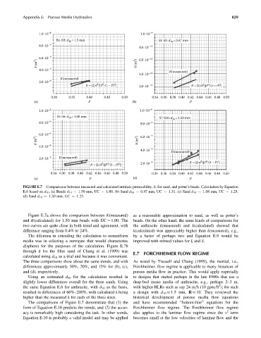
FIGURE E.7 Comparisons between measured and calculated intrinsic permeability, k, for sand, and potter’s beads. Calculation by Equation
E.6 based on d 10 . (a) Beads d 10 ¼ 1.50 mm, UC ¼ 1.00. (b) Sand d 10 ¼ 0.47 mm, UC ¼ 1.31. (c) Sand d 10 ¼ 1.08 mm, UC ¼ 1.25.
(d) Sand d 10 ¼ 1.50 mm, UC ¼ 1.25.

Figure E.7a shows the comparison between K(measured) as a reasonable approximation to sand, as well as potter’s
and K(calculated) for 1.50 mm beads with UC ¼ 1.00. The beads. On the other hand, the same kinds of comparisons for
two curves are quite close in both trend and agreement, with the anthracite k(measured) and k(calculated) showed that
difference ranging from 0.4% to 24%. k(calculated) was appreciably higher than k(measured), e.g.,
The dilemma in extending the calculation to nonuniform by a factor of perhaps two and Equation E.9 would be
media was in selecting a surrogate that would characterize improved with refined values for j and S.
d(sphere) for the purposes of the calculation. Figure E.7b
through d for the filter sand of Chang et al. (1999) was E.7 FORCHHEIMER FLOW REGIME
calculated using d 10 as a trial and because it was convenient.
The three comparisons show about the same trends, and with As noted by Trussell and Chang (1999), the inertial, i.e.,
differences approximately 30%, 20%, and 15% for (b), (c), Forchheimer, flow regime is applicable to many instances of
and (d), respectively. porous media flow in practice. This would apply especially
Using an estimated d 50 for the calculation resulted in to designs that started perhaps in the late 1980s that use a
slightly lower differences overall for the three sands. Using deep-bed mono media of anthracite, e.g., perhaps 2–3m,
2
the same Equation E.6 for anthracite, with d 10 as the basis, with higher HLRs such as say 24 m=h (10 gpm=ft ); for such
resulted in differences of 60%–200%, with calculated k being a design with d 10 1.5 mm, R 10. They reviewed the
higher than the measured k for each of the three sizes. historical development of porous media flow equations
The comparisons of Figure E.7 demonstrate that (1) the and have recommended ‘‘bottom-line’’ equations for the
form of Equation E.10 predicts the trends, and (2) the accur- Forchheimer flow regime. The Forchheimer flow regime
2
acy is remarkably high considering the task. In other words, also applies to the laminar flow regime since the v term
Equation E.10 is probably a valid model and may be applied becomes small at the low velocities of laminar flow and the